De novo identification of microbial contaminants in low microbial biomass microbiomes with Squeegee

Abstract

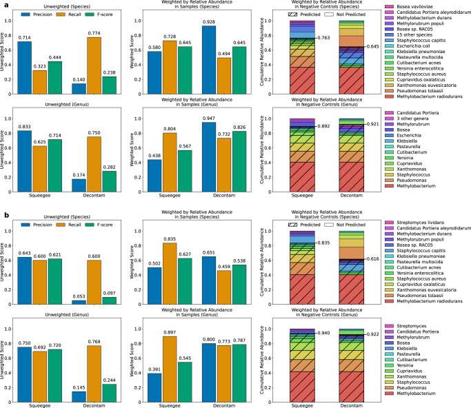
Computational analysis of host-associated microbiomes has opened the door to numerous discoveries relevant to human health and disease. However, contaminant sequences in metagenomic samples can potentially impact the interpretation of findings reported in microbiome studies, especially in low-biomass environments. Contamination from DNA extraction kits or sampling lab environments leaves taxonomic "bread crumbs" across multiple distinct sample types. Here we describe Squeegee, a de novo contamination detection tool that is based upon this principle, allowing the detection of microbial contaminants when negative controls are unavailable. On the low-biomass samples, we compare Squeegee predictions to experimental negative control data and show that Squeegee accurately recovers putative contaminants. We analyze samples of varying biomass from the Human Microbiome Project and identify likely, previously unreported kit contamination. Collectively, our results highlight that Squeegee can identify microbial contaminants with high precision and thus represents a computational approach for contaminant detection when negative controls are unavailable.

Fig. 1. Squeegee pipeline workflow.

Squeegee starts with taxonomic classification using Kraken to determine a set of candidate contaminant species. Reads from the input data are aligned to the representative genomes of the candidate contaminant species using Bowtie2 in multi-alignment mode. It also calculates the pairwise Mash distance for all the samples. Then, it combines the prevalence score, the Mash distance, as well as the breadth/depth of genome coverage of the candidates to predict potential contaminants.

Fig. 2. Benchmarking Squeegee with Decontam on the maternal/infant dataset.

Squeegee (de novo) and Decontam (with negative control) accuracy at species and genus ranks are evaluated with (a) the permissive ground truth and (b) the more strict ground truth. The figures show the precision, recall, and F-score calculated at species and genus rank for both methods. The unweighted precision is calculated as the ratio between the number of predicted contaminant taxa found in the ground truth and the total number of predicted contaminant taxa. The unweighted recall is calculated as the ratio between the number of predicted contaminant taxa found in the ground truth and the total number of taxa in the ground truth. While weighted by samples, the measurements are weighted by the mean proportion of the reads assigned to each taxon in the non-control experiment samples. The weighted by negative controls figures show the detailed composition of the taxa, their mean relative abundance in the negative control samples, and the cumulative relative abundance of the correctly predicted putative contaminants (weighted recall) by different methods. The correctly predicted species/genera are marked with strips, and the species/genera that the methods failed to predict are without stripes. Multiple low relative abundance taxa have been combined in a. Source data are provided as a Source Data file.

Fig. 3. Relative abundance of all predicted species in the maternal/infant dataset.

The samples are clustered by their sample type, which is shown with different colors on the color label on the y-axis. The predicted contaminant species that can be found in the permissive ground truth contaminants are marked by the black label on the x-axis, whereas the predicted contaminant species that do not match the strict ground truth contaminants sample are marked in gray. Source data are provided as a Source Data file.

Fig. 4. Squeegee performance on HMP metagenomic datasets.

a Left panel depicts the Genus level precision, recall, and F-score using previously reported kit contaminants as the ground truth. Unweighted precision is calculated as the ratio between the number of predicted contaminant taxa found in the ground truth and the total number of predicted contaminant taxa. An unweighted recall is calculated as the ratio between the number of predicted contaminant taxa found in the ground truth and the total number of taxa in the ground truth. While weighted by samples, the measurements are weighted by the mean proportion of the reads assigned to each taxon in the non-control experiment samples. b The right panel highlights the correctly predicted genera marked in orange with stripes, and the genera that Squeegee failed to predict are marked in gray. Genera with relative abundance below 1% are combined. Source data are provided as a Source Data file.

Fig. 5. Squeegee prediction accuracy at species ranks on the simulated datasets.

a The leftmost panel shows the precision, recall, and F-score calculated at species rank for the different relative abundance of spike-in contaminants. The unweighted precision is calculated as the ratio between the number of predicted contaminant taxa found in the ground truth and the total number of predicted contaminant taxa. The unweighted recall is calculated as the ratio between the number of predicted contaminant taxa found in the ground truth and the total number of taxa in the ground truth. b The center panel shows the same measurements weighted by the mean proportion of the reads assigned to each taxon in the non-control simulated samples. c The right panel shows the detailed composition of the taxa, their relative abundance in the spike-in contaminant community, and the cumulative relative abundance of the correctly predicted contaminants at a different relative abundance of spike-in. The correctly predicted species are marked with striped lines, and the species Squeegee failed to predict are without striped lines. Source data are provided as a Source Data file.

Fig. 6. Alpha diversity indexes before and after contamination removal.

The figure shows the alpha diversity indexes of a maternal/infant dataset and b HMP dataset. Both Shannon’s and Simpson’s diversity index of the communities in each of the samples were evaluated before the contaminant reads were removed (red), after removing species only confirmed by the experimental negative control (blue), and after removing all species predicted by Squeegee (black). The max removal is set to 1%. Numbers inside parentheses are the numbers of samples in each sample type. The significance test was done using a two-sided Mann–Whitney U–test for all combined sample types with more than 20 samples. No adjustments were made for multiple comparisons. Significance labeling: n.s.(P > 0.05), *(P ≤ 0.05), **(P ≤ 0.01), ***(P ≤ 0.001). Each box plot includes the median line, and the box bounds the interquartile range (IQR). The Tukey-style whiskers extend from the box by at most 1.5 × IQR. The circle denotes outliers that extend beyond the whiskers. In a, the exact p-value between Shannon’s index before removal and reference confirmed contaminants removed is 8.3 × 10⁻⁷ for placenta samples. The exact p-value between Shannon’s index before removal and all contaminants removed is 6.2 × 10⁻⁸ for placenta samples and 1.3 × 10⁻² for breast milk samples. The exact p-value between Simpson’s index before removal and reference confirmed contaminants removed is 9.6 × 10⁻⁵ for placenta samples and 3.8 × 10⁻² for breast milk samples. The exact p-value between Simpson’s index before removal and all contaminants removed is 3.0 × 10⁻⁵ for placenta samples and 1.4 × 10⁻² for breast milk samples. In b, the exact p-value between Shannon’s index before removal and reference confirmed contaminants removed is 2.0 × 10⁻³⁰ for oral samples and 3.0 × 10⁻² for nasal samples. The exact p-value between Shannon’s index before removal and all contaminants removed is 1.0 × 10⁻⁴⁰ for oral samples and 3.7 × 10⁻³ for nasal samples. The exact p-value between Simpson’s index before removal and reference confirmed contaminants removed is 2.0 × 10⁻¹² for oral samples. The exact p-value between Simpson’s index before removal and all contaminants removed is 5.5 × 10⁻¹⁷ for oral samples. Source data are provided as a Source Data file.

References

1. Breitwieser FP, Lu J, Salzberg SL. A review of methods and databases for metagenomic classification and assembly. Brief. Bioinforma. 2019;20:1125–1136. - PMC - PubMed
1. Salter SJ, et al. Reagent and laboratory contamination can critically impact sequence-based microbiome analyses. BMC Biol. 2014;12:87. - PMC - PubMed
1. Davis NM, Proctor DM, Holmes SP, Relman DA, Callahan BJ. Simple statistical identification and removal of contaminant sequences in marker-gene and metagenomics data. Microbiome. 2018;6:226. - PMC - PubMed
1. Fox Gc-a, et al. The phylogeny of prokaryotes. Science. 1980;209:457–463. - PubMed
1. Eckburg PB, et al. Diversity of the human intestinal microbial flora. Science. 2005;308:1635–1638. - PMC - PubMed
Publication types