Bi-EB: Empirical Bayesian Biclustering for Multi-Omics Data Integration Pattern Identification among Species

Abstract

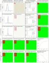
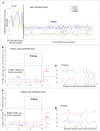
Although several biclustering algorithms have been studied, few are used for cross-pattern identification across species using multi-omics data mining. A fast empirical Bayesian biclustering (Bi-EB) algorithm is developed to detect the patterns shared from both integrated omics data and between species. The Bi-EB algorithm addresses the clinical critical translational question using the bioinformatics strategy, which addresses how modules of genotype variation associated with phenotype from cancer cell screening data can be identified and how these findings can be directly translated to a cancer patient subpopulation. Empirical Bayesian probabilistic interpretation and ratio strategy are proposed in Bi-EB for the first time to detect the pairwise regulation patterns among species and variations in multiple omics on a gene level, such as proteins and mRNA. An expectation-maximization (EM) optimal algorithm is used to extract the foreground co-current variations out of its background noise data by adjusting parameters with bicluster membership probability threshold Ac; and the bicluster average probability p. Three simulation experiments and two real biology mRNA and protein data analyses conducted on the well-known Cancer Genomics Atlas (TCGA) and The Cancer Cell Line Encyclopedia (CCLE) verify that the proposed Bi-EB algorithm can significantly improve the clustering recovery and relevance accuracy, outperforming the other seven biclustering methods-Cheng and Church (CC), xMOTIFs, BiMax, Plaid, Spectral, FABIA, and QUBIC-with a recovery score of 0.98 and a relevance score of 0.99. At the same time, the Bi-EB algorithm is used to determine shared the causality patterns of mRNA to the protein between patients and cancer cells in TCGA and CCLE breast cancer. The clinically well-known treatment target protein module estrogen receptor (ER), ER (p118), AR, BCL2, cyclin E1, and IGFBP2 are identified in accordance with their mRNA expression variations in the luminal-like subtype. Ten genes, including CCNB1, CDH1, KDR, RAB25, PRKCA, etc., found which can maintain the high accordance of mRNA-protein for both breast cancer patients and cell lines in basal-like subtypes for the first time. Bi-EB provides a useful biclustering analysis tool to discover the cross patterns hidden both in multiple data matrixes (omics) and species. The implementation of the Bi-EB method in the clinical setting will have a direct impact on administrating translational research based on the cancer cell screening guidance.

Keywords: biclustering; breast cancer; multi-omics data analysis; tumor and cancer cell lines.

Figure 1

The empirical Bayes model is used to identify the co-regulation biclusters across tumors and cancer cells, both for target module detection. (a) Input data for the Bi-EM algorithm (the row is the gene list, and the column is sample list from different groups or conditions); (b) linear mixture biclustering model illustration (Bi-EM), where the bicluster signals are extracted from background-originating rows and columns, respectively. The mixture model is constructed to identify these biclusters where its grand mean μ₁ is the difference from the background mean μ₂ significantly. (c) Four processing steps of the Bi-EB algorithm. (d) The Bi-EB algorithm searching process. We need to calculate the row and the column possibility in a bicluster and denote each pixel (dot in matrix) in the bicluster as 1 (yes, $\ge Ac$ or 0 (not, $<Ac$) by cut-off $Ac$. The Bi-EB algorithm can identify multiple biclusters sequentially with the associated seed. Each iteration can only identify one bicluster. The bicluster size is based on the number of 1s $>p_{ave}$ (the average possibility of row and column in biclusters). The next bicluster search is based on the left information of rows and columns (the current bicluster outside).

Figure 2

A Bi-EB algorithm for the bicluster on three simulation datasets. (a) The Bi-EB algorithm is tested for the constant-shifted bicluster pattern. (a1,a2) displays a histogram plot and heatmap of the original constant shift bicluster data; (a3) plots the log-likelihood convergence in the EM procedure of Bi-EB in iteration; (a4) displays the extracted bicluster from background using the Bi-EB algorithm. (b) The Bi-EB algorithm is tested on a row-scaled bicluster pattern. (c) The Bi-EB algorithm is tested on column-scaled bicluster data. (b1–c4) have the same description as in (a). (d) The parameter setting of Ac in Bi-EB. (d1–d3) are heatmaps of Bi-EB results with three different values of Ac. (d4) is the sensitivity plot of the Bi-EB algorithm, while the value of Ac changes from 0.2 to 0.09. (e) The parameter setting of p_ave. (e1–e3) are heatmaps of extracted bicluster and (e4) is the accuracy plot of Bi-EB biclusters when the p_ave parameter is set from 0.5 to 0.95.

Figure 3

Bicluster model evaluation. Each group represents the average recovery versus relevance between the TRUE and predicted values in the biclustering algorithms: (a) BI-EB; (b) Bimax; (c) CC; (d) FABIA; (e) Plaid; (f) QUBIC; (g) xMotif; and (h) spectral relevance to constant-shifted, row-scaled, and column-scaled biclusters.

Figure 4

Heat map of membership assignment and extracted biclusters in (a) luminal and (b) basal-like subtypes. (a1,a2) are expression clustering under different conditions to Luminal subtype samples in protein expression data (a1) and mRNA expression data (a2). (a3) is the bi-cluster of ratios of protein amount in (a1) verse mRNA gene expression in (a2) by Bi-EM algorithm. (b1,b2) are expression clustering under different conditions to Basal-like subtype samples in protein expression data (b1) and mRNA gene expression data (b2). (b3) is the bi-cluster of ratios of protein amount in (b1) verse mRNA gene expression in (b2) by Bi-EM algorithm. Red shows the higher probability of belonging to a bicluster and green shows the lower probability of belonging to a bicluster in (a3,b3).

Figure 5

(a) Changes in the mRNA–protein ratio level of all genes across samples in the luminal A/B bicluster in breast cancer. The gray line is the ratio level of the gene in the cancer cell line (CCLE), the yellow line is the ratio level of the gene in tumor TCGA, and the blue line is the ratio level of gene ESR1. (b) The mRNA-protein ratio level of ESR1 across samples in the bicluster. Samples are sorted by ratio measurement. (c) The expression level of gene ESR1 (red) and protein ER (blue) across all samples in the luminal bicluster. Samples keep the same order as in ratio in (b). (d) The mRNA–protein ratio level of ESR1 across 100 samples in the bicluster.

Figure 6

(a) Changes in the mRNA–protein ratio level of all genes across samples in the basal-like bicluster in breast cancer. The blue line is the ratio level of RAB25 and the gold line is CCNB1. (b) The mRNA–protein ratio level of CCNB1 across samples in the bicluster. Samples are sorted by ratio measurement. (c) The expression level of gene CCNB1 (red) and protein (blue) across all samples in the basal-like bicluster. Samples keep the same order as in ratio in (b). (d) The mRNA–protein ratio level of CCNB1 across 34 samples in the bicluster. (e) The mRNA–protein ratio level of RAB25 across samples in the bicluster. Samples are sorted by ratio measurement. (f) The expression level of gene RAB25 (red) and protein (blue) across all samples in the basal-like bicluster. Samples keep the same order as in ratio in (e). (g) The mRNA–protein ratio level of RAB25 across 34 samples in the bicluster.

References

-
- Saber H.B., Elloumi M. DNA microarray data analysis: A new survey on biclustering. Int. J. Comput. Biol. 2015;4:21–37. doi: 10.34040/IJCB.4.1.2014.36. - DOI
- Cheng Y., Church G.M. Biclustering of expression data. Proc. Int. Conf. Intell. Syst. Mol. Biol. 2000;8:93–103. - PubMed
- Lazzeroni L., Owen A. Plaid models for gene expression data. Stat. Sin. 2002;12:61–86.
Publication types
MeSH terms
Substances
Grants and funding
LinkOut - more resources
Full Text Sources
Medical
Research Materials
Miscellaneous