Crosshair, semi-automated targeting for electron microscopy with a motorised ultramicrotome

Abstract

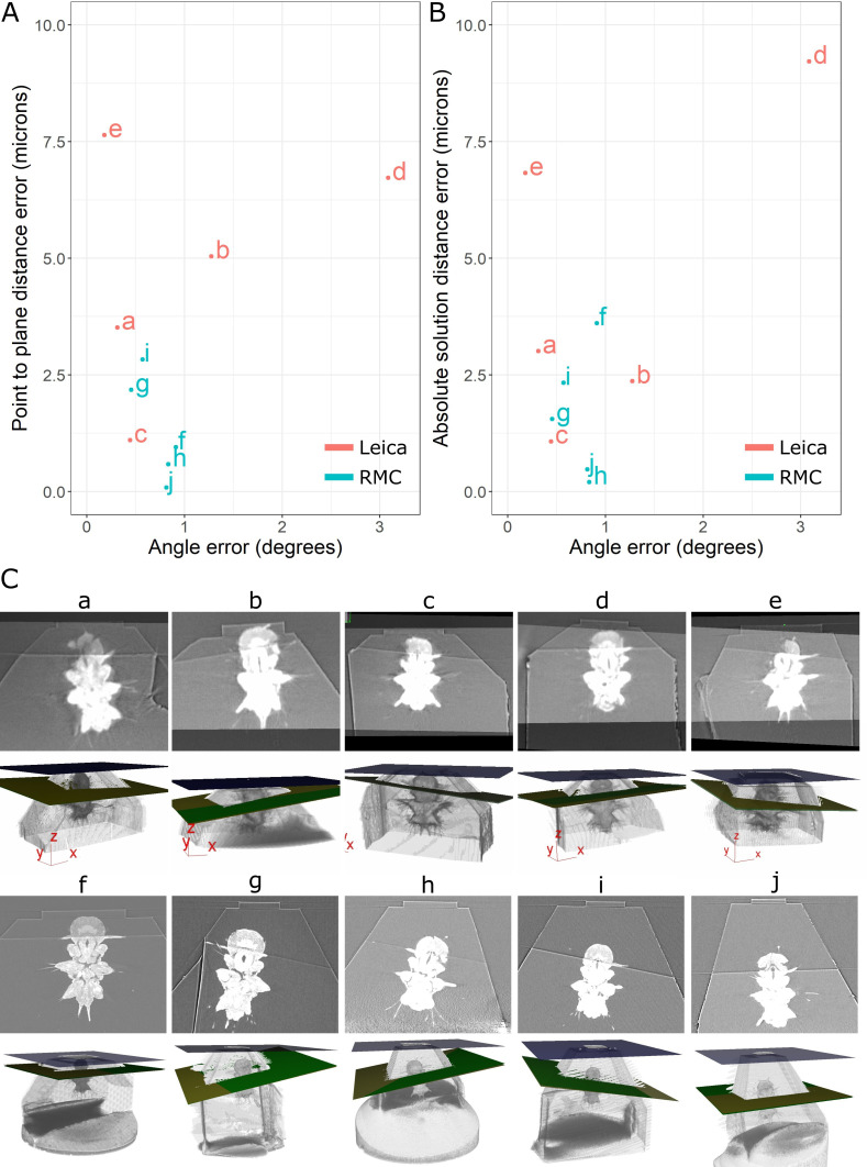
Volume electron microscopy (EM) is a time-consuming process - often requiring weeks or months of continuous acquisition for large samples. In order to compare the ultrastructure of a number of individuals or conditions, acquisition times must therefore be reduced. For resin-embedded samples, one solution is to selectively target smaller regions of interest by trimming with an ultramicrotome. This is a difficult and labour-intensive process, requiring manual positioning of the diamond knife and sample, and much time and training to master. Here, we have developed a semi-automated workflow for targeting with a modified ultramicrotome. We adapted two recent commercial systems to add motors for each rotational axis (and also each translational axis for one system), allowing precise and automated movement. We also developed a user-friendly software to convert X-ray images of resin-embedded samples into angles and cutting depths for the ultramicrotome. This is provided as an open-source Fiji plugin called Crosshair. This workflow is demonstrated by targeting regions of interest in a series of Platynereis dumerilii samples.

Keywords: P. dumerilii; cell biology; electron microscopy; open-source software; targeted acquisition.

Figure 1.. Motorised ultramicrotome.

(A) Summary of the main ultramicrotome axes of rotation (sample tilt, sample rotation, and knife tilt), and movement (north–south [NS]/east–west [EW]), which are common to both Leica and RMC systems. (B) Overview of motorised Leica system. (C) Overview of motorised RMC system. (D) Zoom of (B), showing motors attached to each axis. (E) Zoom of (C), showing motors attached to each axis.

Figure 1—figure supplement 1.. Motorised ultramicrotomes and user interfaces.

(A) Leica ultramicrotome arm with sample holder removed. This shows the additional hole that was drilled (here there are three holes, but the top labelled one is the only required). (B) Zoom of the back of the Leica sample holder, showing the small metal pin that was added to fit into the hole in (A). (C) Knife tilt page of the user interface for the motorised Leica system. This is shown on a touchscreen to the right of the ultramicrotome and allows motors to be enabled/disabled and set to specific angles. (D) User interface of the motorised RMC system.

Figure 1—figure supplement 2.. Calibration of sample tilt axis.

(A) Diagram of calibration setup, with RMC system. (B) Graph of sample tilt vs. motor steps for RMC system. A linear fit is shown in red. (C) Same as (B) for Leica system.

Figure 1—figure supplement 3.. Calibration of sample rotation axis.

(A) Diagram of calibration setup, with RMC system. (B) Graph of sample rotation vs. motor steps for RMC system. A linear fit is shown in red. (C) Same as (B) for Leica system.

Figure 1—figure supplement 4.. Calibration of knife tilt axis.

(A) Diagram of calibration setup, with RMC system. (B) Graph of knife tilt vs. motor steps for RMC system. A linear fit is shown in red. (C) Same as (B) for Leica system.

Figure 2.. Targeting problem.

(A) Left: diagram of a resin block with a Platynereis sample inside. The top surface has been trimmed flat with a diamond knife. Right: same resin block with labelled block plane (i.e. the plane parallel to the flat trimmed surface) and target plane. (B) Diagram of the block in the ultramicrotome before (left) and after (right) the orientation solution is applied. A top view (with diamond knife at the bottom, and sample holder at the top) and side view (with diamond knife on the left, and sample holder on the right) are shown. ${\theta }_K$ is the knife tilt angle, ${\theta }_T$ is the sample tilt angle, and ${\theta }_R$ is the sample rotation angle. (C) Diagram of the block in the ultramicrotome before (left) and after (right) the distance solution is applied. Top/side view are the same as in (B). $D_{NS}$ is the NS cutting distance.

Figure 3.. Coordinate frames, pose diagrams, and solutions.

(A) Diagram of all coordinate frames. World: x is parallel to EW, y is parallel to NS, z is vertical. Knife: z points out of the page, and is parallel to the world frame z. Arc: x is parallel to the world frame x. Holder: y points into the page and is parallel to the arc frame y. Block: x is parallel to the bottom edge of the block face. Two variations are shown: a rectangular block face (left) and a trapezium block face (right). Target: y is perpendicular to the target plane (shown in grey). (B) Diagram of relation between block and target coordinate frames. Left: 3D view of the block, showing the block frame (red) and target plane (grey). Middle: 2D view of the block frame’s xy plane (i.e. looking down on the block from above). The target plane intersects along the shown grey line, and ${\theta }_{to}$ is the angle between the red and blue x axes, that is, the rotation angle about the block frame z. Right: 2D view of the blue axes’ zy plane (i.e. looking down the line of intersection from the middle panel). ${\theta }_{tr}$ is the angle between the blue and green z axes, that is, the rotation angle about the blue frame x. The green axes are the final target coordinate frame (as shown in A). (C) Pose diagram showing relations between coordinate frames. $R_x$, $R_y$, $R_z$: rotation matrices about the x, y, and z axes, respectively; ${\theta }_T$: sample tilt angle; ${\theta }_R$: sample rotation angle; ${\theta }_K$: knife angle; ${\theta }_{to}$: target offset angle; ${\theta }_{tr}$: target rotation angle. Dashed arrows are unknown relations. (D) Pose diagram when the knife is aligned to the block face. Here, the knife frame is in the same orientation as the block (red arrow), and therefore we can infer the Holder to Block relation that was unknown in (C). ${\theta }_{IT}$ is the initial sample tilt angle and ${\theta }_{IK}$ is the initial knife tilt angle, when the knife and block are aligned. We define ${\theta }_R$ to be zero at this aligned orientation. (E) Graphs of knife and sample tilt solution for all sample rotation angles. This used values of ${\theta }_{IK}$ = 10, ${\theta }_{IT}$ = 10, ${\theta }_{to}$ = –3.3, and ${\theta }_{tr}$ = 5.4. (F) Solution graphs with more extreme initial angles. ${\theta }_{IK}$ = 10, ${\theta }_{IT}$ = 10, ${\theta }_{to}$ = –60, and ${\theta }_{tr}$ = 5.4.

Figure 3—figure supplement 1.. Coordinate frames at different angles.

(A) Knife coordinate frame at 0° (top) and 10° (bottom). Note that at 0° the knife frame has the same orientation as the world frame. (B) Arc coordinate frame at 0° (top) and 14° (bottom). Note that at 0° the arc frame has the same orientation as the world frame. (C) Holder coordinate frame at two positions separated by a 90° rotation. Note that here the 0 position depends on the particular targeting run as it is defined as the rotation when the knife and block face are aligned.

Figure 3—figure supplement 2.. Distance calculation.

Here, the same block and target plane as in Figure 3B are shown in an example solution orientation. In red is the World coordinate frame, showing we are looking down the world z-axis. The knife is aligned to the vertical target plane, but the ultramicrotome arm (and therefore the block) advances towards the knife in the world y-axis (NS) between cuts. Therefore, the required cutting distance is not the same as the perpendicular distance between the knife and target plane. $D_P$ is the perpendicular distance between the target plane and the furthest surface point, $D_{NS}$ is the corresponding NS distance (i.e. the required cutting depth), and ${\theta }_K$ is the knife angle.

Figure 4.. Targeting workflow.

Summary of targeting workflow steps with representative images/3D renders.

Figure 5.. Crosshair.

(A) Crosshair plugin user interface, with an example Platynereis dumerilii X-ray image. Left: controls; middle: BigDataViewer window showing 2D cross-section. Right: ImageJ 3D viewer showing volume rendering with block and target planes (blue and green, respectively). The green target plane is the same as the 2D slice shown. (B) Left: microtome mode controls and solution display. Right: corresponding 3D representation of ultramicrotome and sample.

Figure 5—figure supplement 1.. Crosshair user interface.

Crosshair. Left column: 2D slice. Right column: 3D volume rendering. (A) Three points placed on the block surface to fit a plane. (B) Block surface shown in 2D and 3D (blue plane) with labelled corners and orientation. The green points in the 2D view are the points used to fit the plane originally. (C) Example of ‘cutting mode’. The 2D slice shows the predicted surface at a certain cut depth, indicated in 3D by the large pink plane.

Figure 6.. Accuracy test results.

(A) Graph of point-to-plane distance error vs. angle error for all 10 samples (a–j). (B) Graph of absolute solution distance error vs. angle error. (C) For each sample (a–j), two images are shown. Top: registered before and after X-ray images. Bottom: snapshot of the 3D viewer in Crosshair. In the 3D view, the block surface is shown in blue, the target in green, and the plane reached in yellow. In most cases, the green and yellow planes are too close together to distinguish well. The axes shown in some of these images are the 3D viewer coordinate system.

Figure 6—figure supplement 1.. Registration accuracy.

(A) Beeswarm plot of distance error (microns) measured between manually placed corresponding points on pairs of registered X-ray images for samples (a–j). Two repeats of manually placing points in the same locations on the same images are shown. (B) Absolute difference (microns) between the distance error measured in (A) between repeat 1 and repeat 2 for each point.

Figure 6—figure supplement 2.. Sample mounting for trimming, X-ray imaging, and targeting for samples f–j.

(A) Resin-embedded sample mounted onto an aluminium pin using conductive epoxy glue. (B) An aluminium pin with sample inserted into a Gatan Rivet Holder which is directly inserted into an ultramicrotome chuck holder for trimming and targeting at the ultramicrotome. (C) An aluminium pin with sample mounted to a sample holder of Versa 510 X-ray microscope for X-ray imaging.

Figure 7.. Comparison of target plane (from the before scan) to the block surface (after scan).

Each sample (a–j) has a column with three images. Top row: the target plane from the before targeting scan. Middle row: the block surface from the after targeting scan. Bottom row: cross-section parallel to block surface, but 3 µm inside the block. The middle row images can be quite dark/noisy as they slice right along the surface of the block, so the bottom row is provided so the cross-section can be seen more easily.

Figure 7—figure supplement 1.. Comparison of example Platynereis X-ray cross-sections, both acquired with 1 micron isotropic voxel size.

(A) Sample d X-ray, acquired with Bruker SkyScan 1272 (system used for samples a–e). (B) Sample f X-ray, acquired with Zeiss Versa 510 (system used for samples f–j). Note the sharper block edges and the finer anatomical details visible in (B).

References

1. Baena V, Schalek RL, Lichtman JW, Terasaki M. Serial-section electron microscopy using automated tape-collecting ultramicrotome (ATUM) Methods in Cell Biology. 2019;152:41–67. doi: 10.1016/bs.mcb.2019.04.004. - DOI - PMC - PubMed
1. Bogovic JA, Hanslovsky P, Wong A, Saalfeld S. Robust registration of calcium images by learned contrast synthesis. 2016 IEEE 13th International Symposium on Biomedical Imaging (ISBI 2016; Prague, Czech Republic. 2016. pp. 1123–1126. - DOI
1. Bosch C, Ackels T, Pacureanu A, Zhang Y, Peddie CJ, Berning M, Rzepka N, Zdora MC, Whiteley I, Storm M, Bonnin A, Rau C, Margrie T, Collinson L, Schaefer AT. Functional and multiscale 3D structural investigation of brain tissue through correlative in vivo physiology, synchrotron micro-tomography and volume electron microscopy. Nature Communications. 2022;13:2923. doi: 10.1038/s41467-022-30199-6. - DOI - PMC - PubMed
1. Brama E, Peddie CJ, Wilkes G, Gu Y, Collinson LM, Jones ML. UltraLM and minilm: locator tools for smart tracking of fluorescent cells in correlative light and electron microscopy. Wellcome Open Research. 2016;1:26. doi: 10.12688/wellcomeopenres.10299.1. - DOI - PMC - PubMed
1. Bushong EA, Johnson DD, Kim KY, Terada M, Hatori M, Peltier ST, Panda S, Merkle A, Ellisman MH. X-ray microscopy as an approach to increasing accuracy and efficiency of serial block-face imaging for correlated light and electron microscopy of biological specimens. Microscopy and Microanalysis. 2015;21:231–238. doi: 10.1017/S1431927614013579. - DOI - PMC - PubMed
Publication types