Mathematical Foundations of Adaptive Isogeometric Analysis

Abstract

This paper reviews the state of the art and discusses recent developments in the field of adaptive isogeometric analysis, with special focus on the mathematical theory. This includes an overview of available spline technologies for the local resolution of possible singularities as well as the state-of-the-art formulation of convergence and quasi-optimality of adaptive algorithms for both the finite element method and the boundary element method in the frame of isogeometric analysis.

Fig. 1

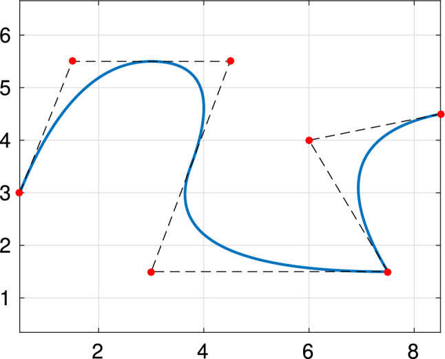
Quadratic spline curve, constructed from the knot vector $T=(0,0,0,1/4,2/4,3/4,3/4,1,1,1)$, along with its control points in ${\mathbb{R}}^2$

Fig. 2

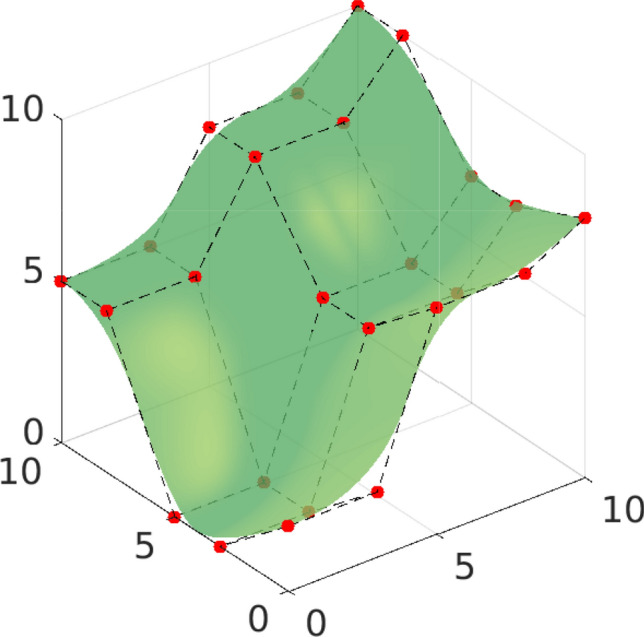
Quadratic spline surface, constructed from the knot vectors $T_1=T_2=(0,0,0,1/3,2/3,1,1,1)$, along with its control points in ${\mathbb{R}}^3$

Fig. 3

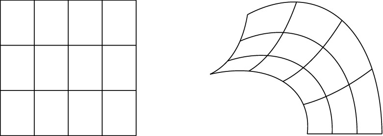
Mesh in the parametric domain (left) and its image through $\mathbf{F}$ in the physical domain (right)

Fig. 4

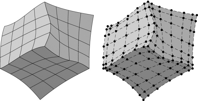
An example of a multi-patch domain formed by three patches (left), and their corresponding control points (right). The control points associated to interface functions of adjacent patches coincide

Fig. 5

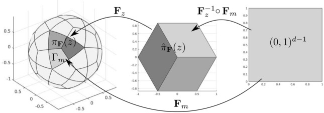
Graphical representation of assumption (P3), in a parametrization of the sphere with 60 patches and one single element per patch. The three elements forming ${\pi }_{\mathbf{F}}(\mathbf{z})$ on the left are colored in different tones of gray, and the corresponding polygon ${\widehat{\pi }}_{\mathbf{F}}(\mathbf{z})$ is the hexagon shown in the middle. The mapping ${\mathbf{F}}_{\mathbf{z}}^{-1}\circ {\mathbf{F}}_m$ is an affine transformation

Fig. 6

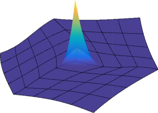
An example of a $C^0$ basis function of the multi-patch space, defined in the same domain as in Fig. 4

Fig. 7

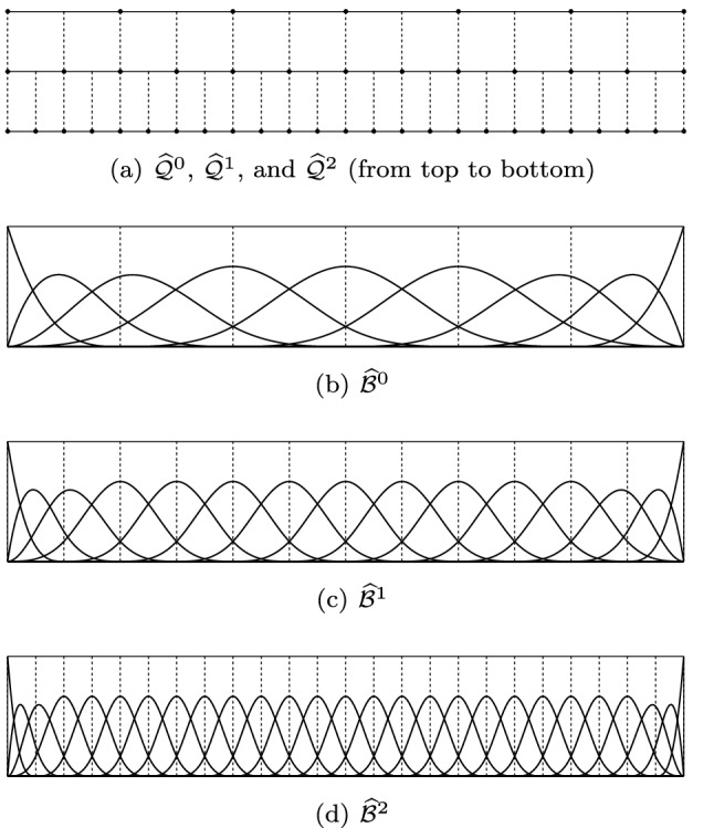
An example of grids (a) of three hierarchical levels for $\widehat{d}=1$. The univariate B-splines of degree 3 defined on level 0, 1 and 2 are shown in (b–d), respectively. All internal knots have multiplicity one

Fig. 8

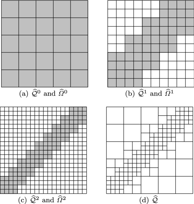
An example of grids and domains (gray regions) of levels 0 (a), 1 (b), 2 (c) for $\widehat{d}=2$. The hierarchical mesh is also shown (d)

Fig. 9

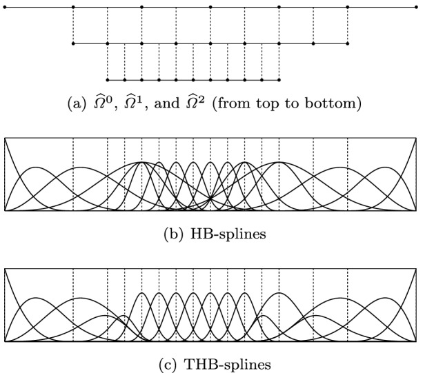
An example of cubic HB-splines (b) and THB-splines (c) defined on a domain hierarchy consisting of three levels (a). All internal knots have multiplicity one

Fig. 10

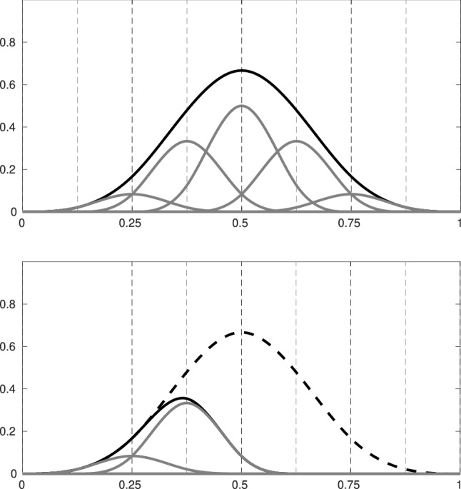
Top: a univariate cubic B-spline of level $\ell$ (in black) represented as linear combination of functions of level $\ell +1$ (in gray). Bottom: the original B-spline (solid dashed) and its truncated version (black solid line) by considering ${\Omega }^{\ell +1}=[0.25,1]$

Fig. 11

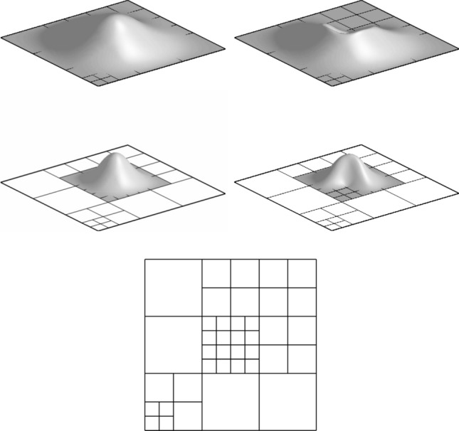
Two bi-quadratic mother B-splines (left) and corresponding THB splines (right) defined on a hierarchical mesh with three levels (bottom). All internal knots have multiplicity one

Fig. 12

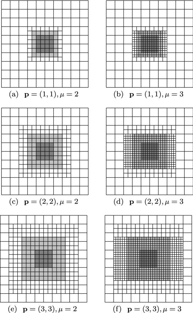
Examples of the domains ${\widehat{\omega }}_{\mathcal{H}}^1$ (dark gray) and ${\widehat{\omega }}_{\mathcal{T}}^1$ (light gray) for different degrees and mesh configurations. All internal knots have multiplicity one

Fig. 13

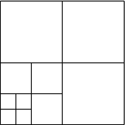
A $\mathcal{T}$-admissible mesh for $\mathbf{p}=(1,1)$ and $\mu =2$ with three levels: HB-splines of level 0, 1, 2 are non zero on the element of the finest level in the bottom left corner. THB-splines of only levels 1, 2 are non zero on the same element

Fig. 14

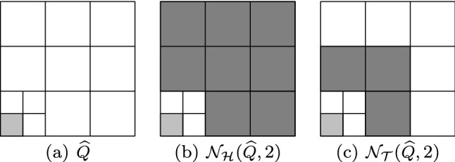
For the light gray element $\widehat{Q}$ (a), we plot in dark gray its $\mathcal{H}$-neighborhood (b) and $\mathcal{T}$-neighborhood (c), for $\mathbf{p}=(2,2)$ and $\mu =2$. All internal knots have multiplicity one

Fig. 15

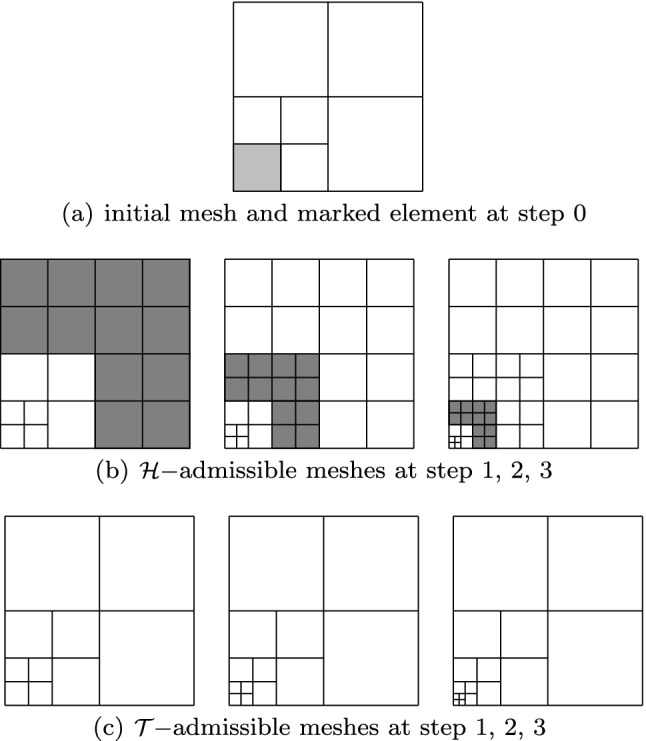
$\mathcal{H}$-admissible (b) and $\mathcal{T}$-admissible (c) meshes generated by Algorithm 1 and 2, respectively, by refining three times the finest element in the bottom left corner of the mesh with $\mathbf{p}=(1,1)$ and $\mu =2$. The initial mesh and a marked element at step 0 are shown as well (a). At each step, the dark gray elements appear by refinement of the neighborhood of the previous marked element. All internal knots have multiplicity one

Fig. 16

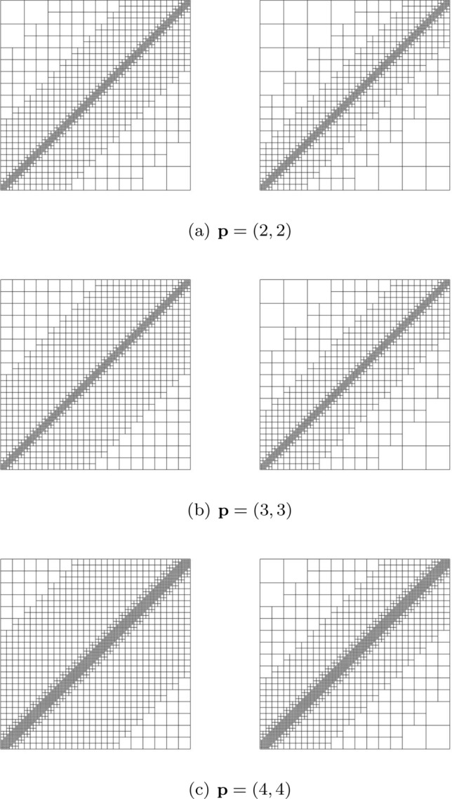
Diagonal refinement of the unit square, starting from a uniform $4\times 4$ mesh, after six refinement steps: $\mathcal{H}$-admissible (left) and $\mathcal{T}$-admissible (right) meshes generated by Algorithm 1 and 2, respectively. Results for $\mu =3$ and $\mathbf{p}=(2,2)$, $\mathbf{p}=(3,3)$, $\mathbf{p}=(4,4)$. At each refinement step, we mark a strip of $2\lceil \frac{p+1}{2}\rceil$ cells centered at the diagonal. This naturally guarantees that in each step functions of the finest level are activated. All internal knots have multiplicity one

Fig. 17

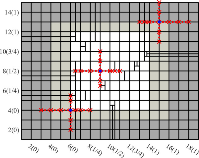
A two-dimensional T-mesh with degree $(p_1,p_2)=(5,3)$. For the three (blue) nodes $\mathbf{z}\in \{(6,4),(9,8),(15,13)\}$, their corresponding local knot vectors are indicated by red crosses. In the axes we indicate the indices in ${\mathcal{I}}_j^0$ and, between parentheses, the value of the corresponding knots. (Color figure online)

Fig. 18

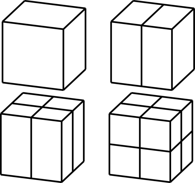
Example of bisection for $\widehat{d}=2$. The initial element of level 0 is bisected in the x-direction ($\mathrm{dir}(0)=1$) to obtain two elements of level 1. These are then bisected in the y-direction ($\mathrm{dir}(1)=2$) to obtain the four elements of level 2

Fig. 19

Example of bisection for $\widehat{d}=3$. The initial element of level 0 is bisected in the x-direction ($\mathrm{dir}(0)=1$) to obtain two elements of level 1. These are then bisected in the y-direction ($\mathrm{dir}(1)=2$) to obtain four elements of level 2, which are bisected in the z-direction ($\mathrm{dir}(2)=3$) to get eight elements of level 3

Fig. 20

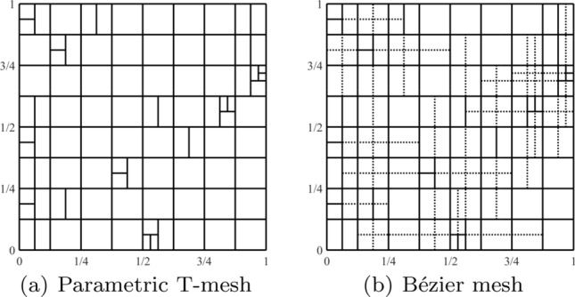
Parametric T-mesh and corresponding Bézier mesh, for the index T-mesh in Fig. 17 and degree $\mathbf{p}=(5,3)$

Fig. 21

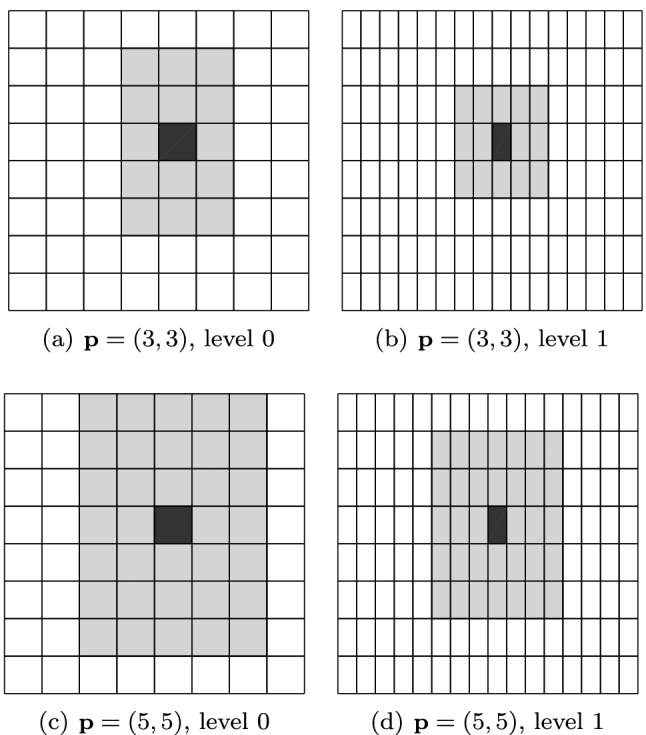
Visualization of the generalized neighborhood on uniform leveled meshes, for simplicity represented in ${\check{\Omega }}_{\mathrm{ip}}$, and for different degrees. For the element $\check{Q}$ in dark gray, its generalized neighborhood ${\mathcal{N}}^{\mathrm{gen}}(\check{Q})$ is formed by all the gray elements

Fig. 22

Visualization of the generalized neighborhood for degree $\mathbf{p}=(5,3)$ in $\widehat{\Omega }$. For the element $\widehat{Q}$ in dark gray, its generalized neighborhood ${\mathcal{N}}^{\mathrm{gen}}(\widehat{Q})$ is formed by all the gray elements, while the neighborhood $\mathcal{N}(\widehat{Q})$ is constituted only by the light gray elements

Fig. 23

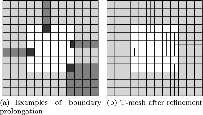
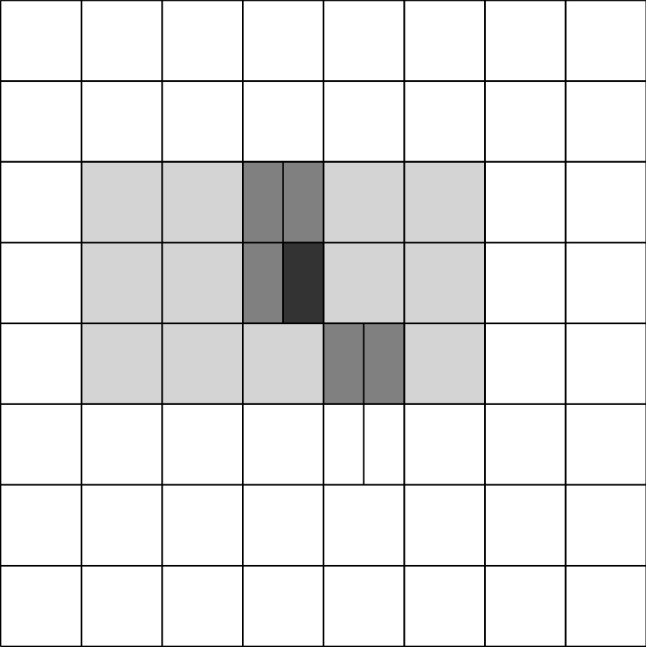
The left figure shows the boundary prolongations of the dark gray elements, which are given by the gray elements. The right figure shows the result of applying Algorithm 3, after marking the dark gray elements on the left figure. The degree is $p_1=p_2=3$. Light gray elements are outside ${\check{\Omega }}_{\mathrm{ip}}$

Fig. 24

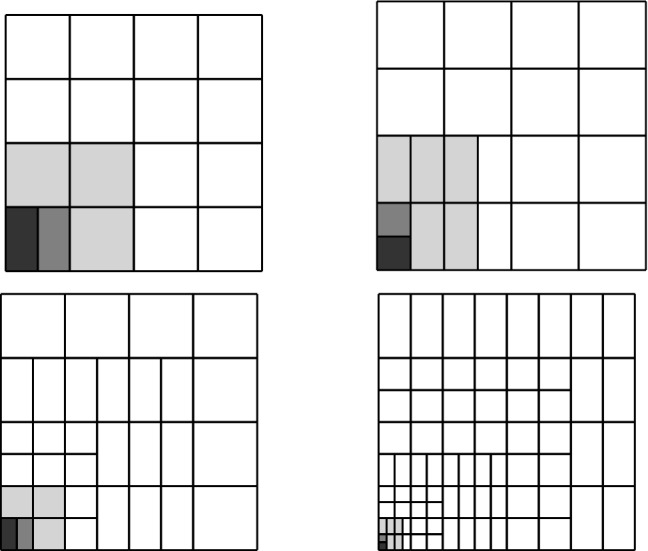
Application of Algorithm 4 starting from a $4\times 4$ parametric T-mesh, with degree $\mathbf{p}=(5,3)$, and marking always the element in the bottom left corner. The plot shows the refined parametric T-meshes after 1, 2, 3, and 6 refinement steps. The marked element $\widehat{Q}$ is highlighted in dark gray, while all the elements in gray belong to its generalized neighborhood ${\mathcal{N}}^{\mathrm{gen}}(\widehat{Q})$, and the elements in light gray belong to its neighborhood $\mathcal{N}(\widehat{Q})$, and therefore are marked by the refinement algorithm. Note that also the neighbors of these elements, which we do not highlight, are marked for refinement by the algorithm

Fig. 25

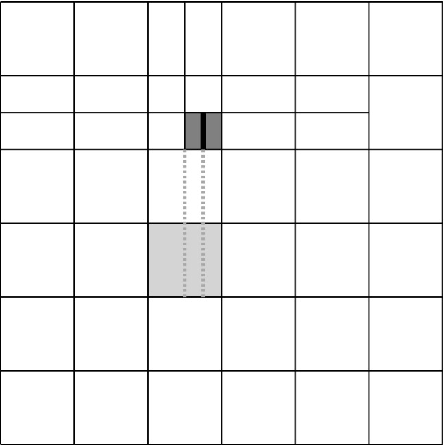
For degree $\mathbf{p}=(3,3)$, the element $\check{Q}$ (light gray) is bisected in more than two Bézier elements after the bisection of ${\check{Q}}^{\prime }$ (dark gray). The element ${\check{Q}}^{\prime }$ is bisected by the thick black line in direction $s=1$, and it is translated with respect to $\check{Q}$ in direction $\tilde{s}=2$

Fig. 26

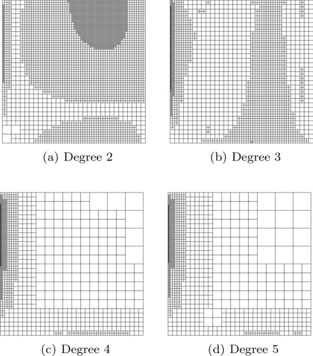
Test with edge singularities: meshes obtained after 15 iterations of the adaptive algorithm for $\mathcal{T}$-admissible meshes and $\mu =2$

Fig. 27

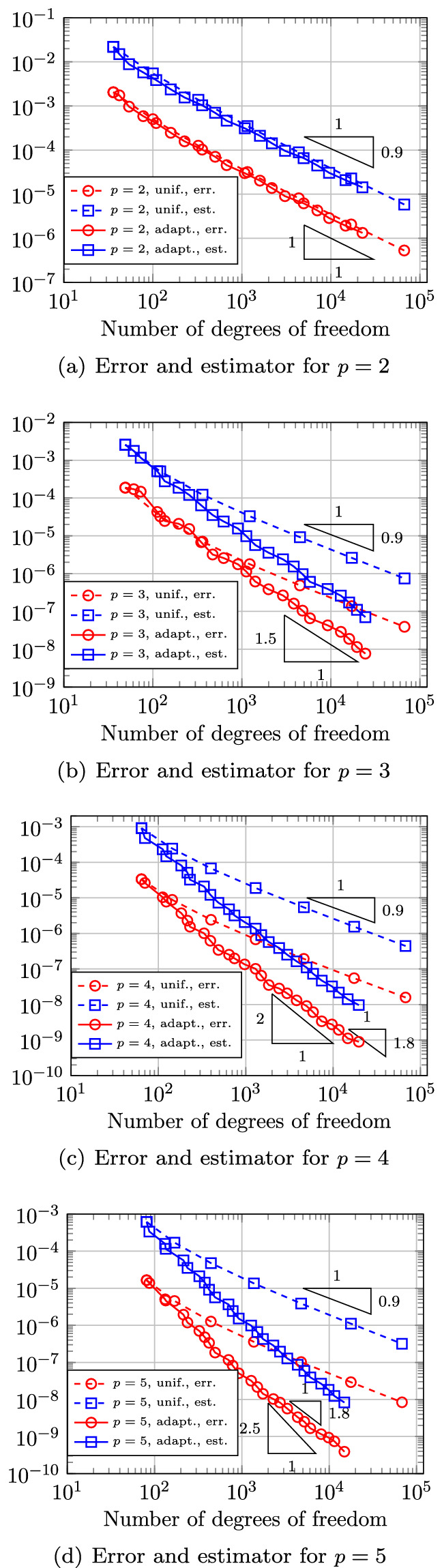
Test with edge singularities: energy error $|u-U_k{|}_{H^1(\Omega )}$ and residual estimator for degree $p\in \{2,3,4,5\}$. Comparison of uniform and adaptive refinement

Fig. 28

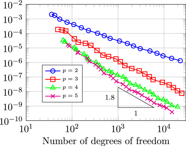
Test with edge singularities: energy error $|u-U_k{|}_{H^1(\Omega )}$ for degree p from 2 to 5. For high degree, the optimal convergence rate is not reached

Fig. 29

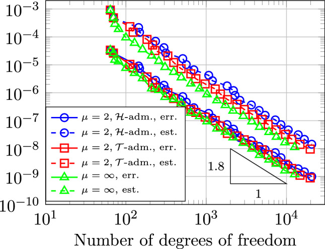
Test with edge singularities: residual estimator and energy error $|u-U_k{|}_{H^1(\Omega )}$ for degree $p=4$. Results for $\mathcal{H}$-admissible and $\mathcal{T}$-admissible meshes of class $\mu =2$, and for non-admissible meshes

Fig. 30

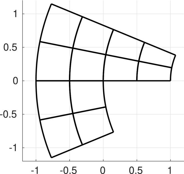
Curved L-shaped domain: domain and initial mesh

Fig. 31

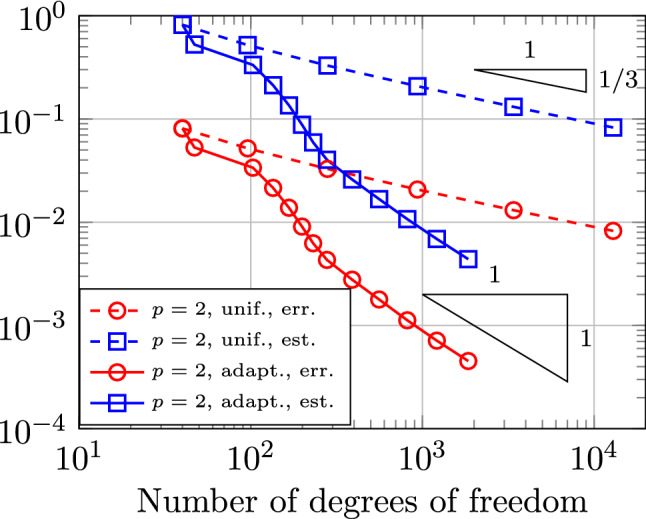
Curved L-shaped domain: energy error and residual estimator for degree $p=2$, for uniform refinement and adaptive refinement on $\mathcal{T}$-admissible meshes with $\mu =2$

Fig. 32

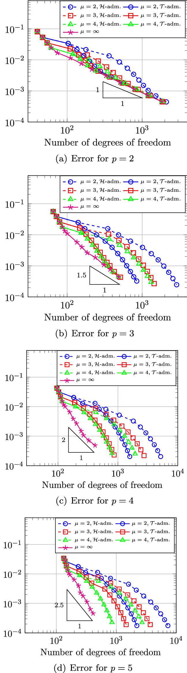
Curved L-shaped domain: energy error $|u-U_k{|}_{H^1(\Omega )}$ for degree p from 2 to 5, and for different values of the admissibility class $\mu$, both for $\mathcal{H}$-admissible and $\mathcal{T}$-admissible meshes

Fig. 33

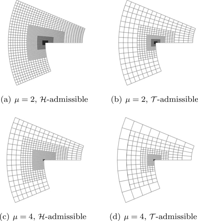
Curved L-shaped domain: mesh after 8 refinement steps for degree $p=4$

Fig. 34

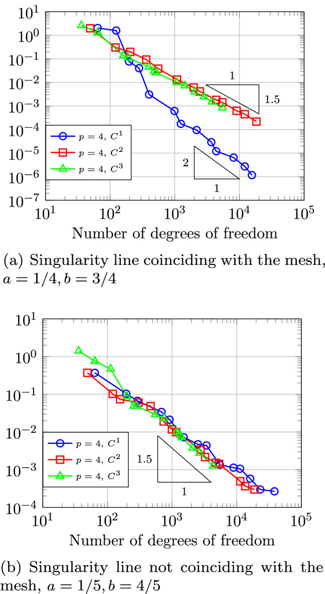
Test about the approximation class: energy error $|u-U_k{|}_{H^1(\Omega )}$ for degree $p=4$ and $\mathcal{T}$-admissible meshes with $\mu =4$, with THB-splines of different continuity

Fig. 35

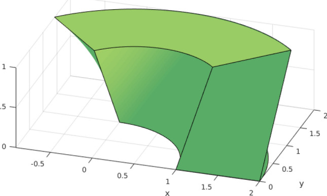
Twisted thick ring: coordinates of the domain

Fig. 36

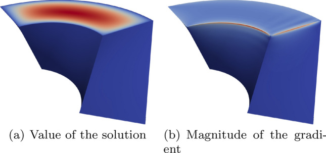
Twisted thick ring: approximate solution and the magnitude of the gradient

Fig. 37

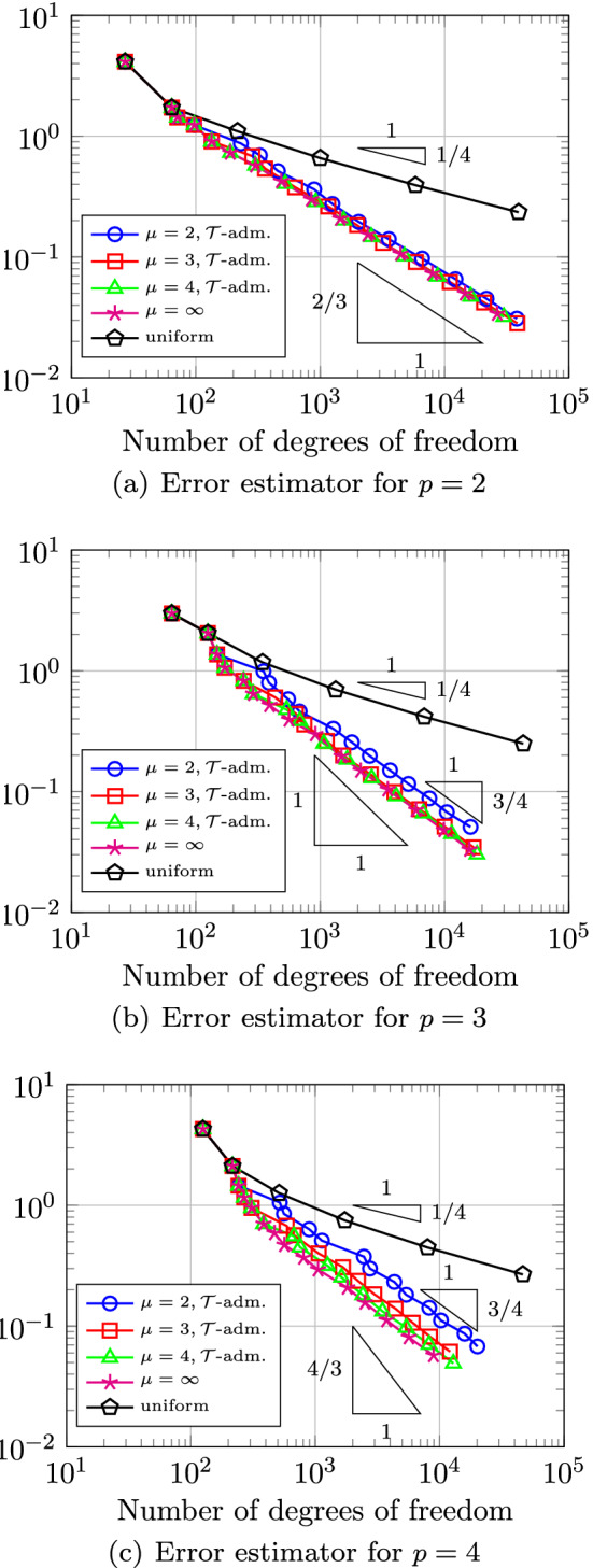
Twisted thick ring: comparison of the error estimator for uniform refinement and adaptive refinement with different degree p and admissibility class $\mu$

Fig. 38

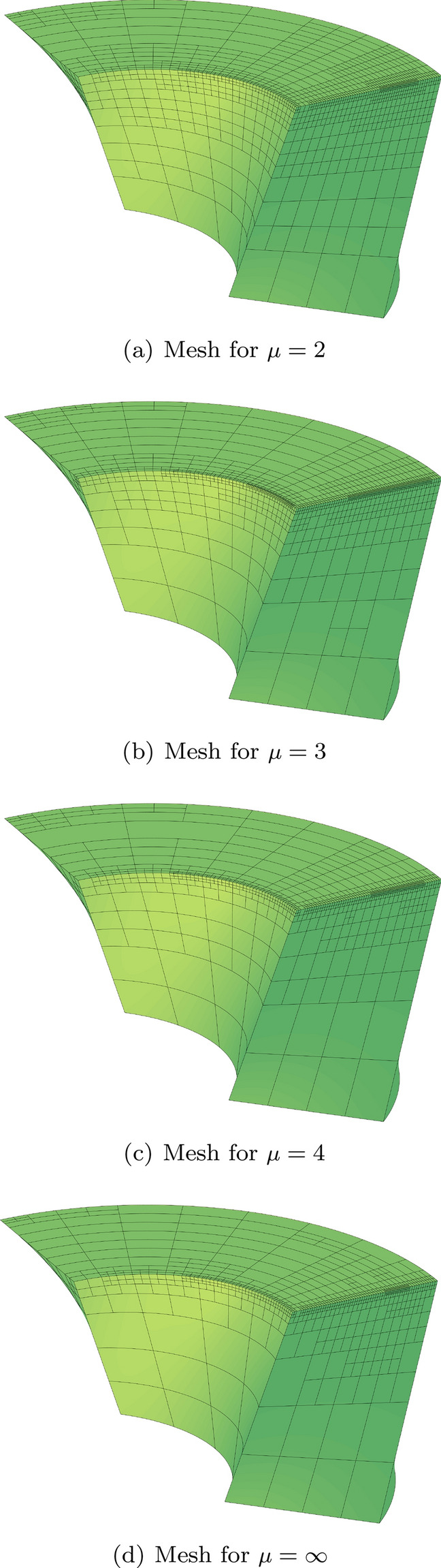
Twisted thick ring: meshes for degree $p=3$ and different values of the admissibility class $\mu$ after eight refinement steps

Fig. 39

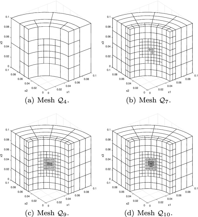
Quasi-singularity on thick ring: Hierarchical meshes generated by Algorithm 5 (with $\theta =0.5$) for hierarchical splines of degree $p=1$

Fig. 40

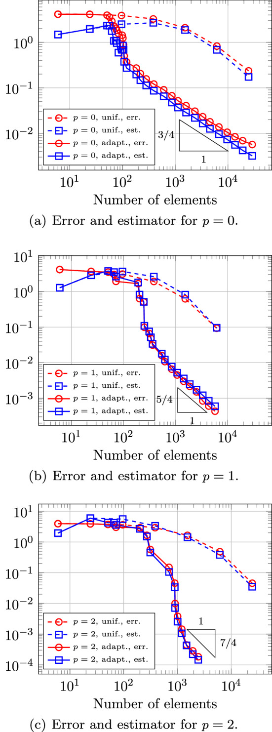
Quasi-singularity on thick ring: Energy error $\Vert \varphi -{\Phi }_k{\Vert }_{\mathcal{V}}$ and estimator ${\eta }_k$ of Algorithm 5 for hierarchical splines of degree p are plotted versus the number of elements $\#{\mathcal{Q}}_k$. Uniform and adaptive ($\theta =0.5$) refinement is considered

Fig. 41

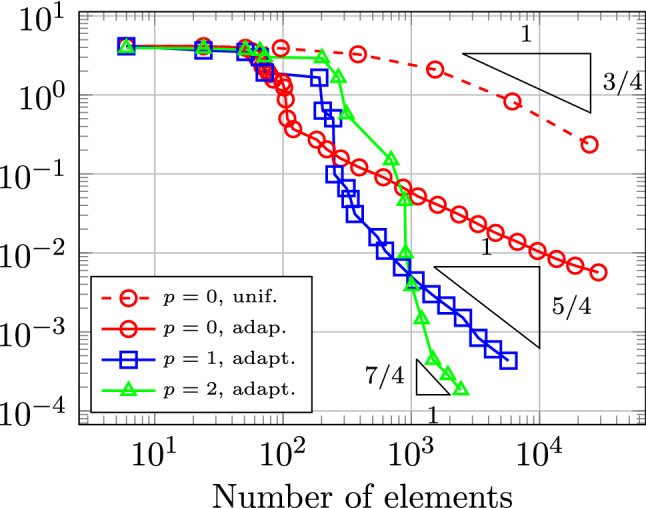
Quasi-singularity on thick ring: The energy errors $\Vert \varphi -{\Phi }_k{\Vert }_{\mathcal{V}}$ of Algorithm 5 for hierarchical splines of degree $p\in \{0,1,2\}$ are plotted versus the number of elements $\#{\mathcal{Q}}_k$. Uniform (for $p=2$) and adaptive ($\theta =0.5$ for $p\in \{0,1,2\}$) refinement is considered

Fig. 42

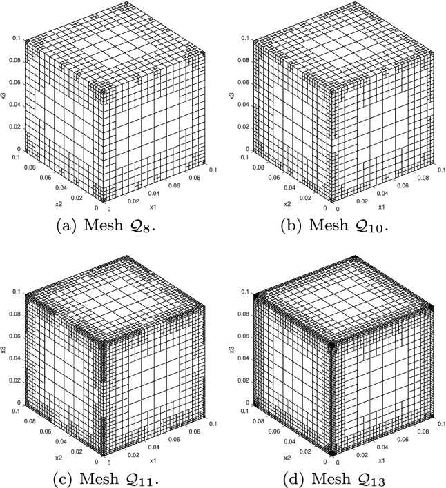
Exterior problem on cube: Hierarchical meshes generated by Algorithm 5 (with $\theta =0.5$) for hierarchical splines of degree $p=1$

Fig. 43

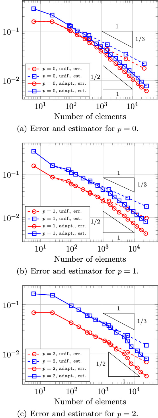
Exterior problem on cube: Energy error $\Vert \varphi -{\Phi }_k{\Vert }_{\mathcal{V}}$ and estimator ${\eta }_k$ of Algorithm 5 for hierarchical splines of degree p are plotted versus the number of elements $\#{\mathcal{Q}}_k$. Uniform and adaptive ($\theta =0.5$) refinement is considered

Fig. 44

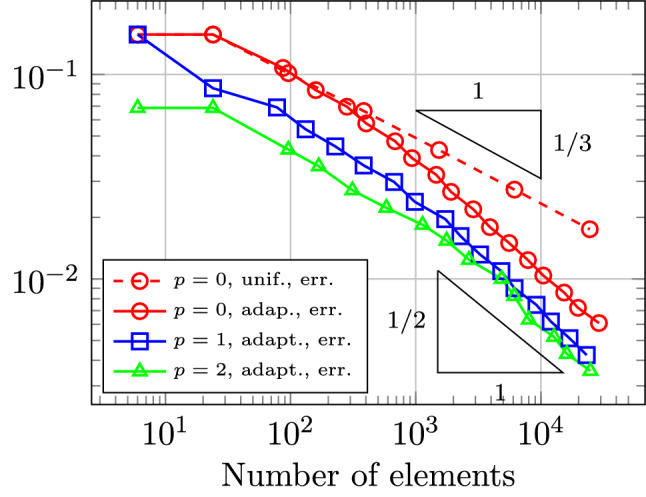
Exterior problem on cube: The energy errors $\Vert \varphi -{\Phi }_k{\Vert }_{\mathcal{V}}$ of Algorithm 5 for hierarchical splines of degree $p\in \{0,1,2\}$ are plotted versus the number of elements $\#{\mathcal{Q}}_k$. Uniform (for $p=0$) and adaptive ($\theta =0.5$ for $p\in \{0,1,2\}$) refinement is considered

Fig. 45

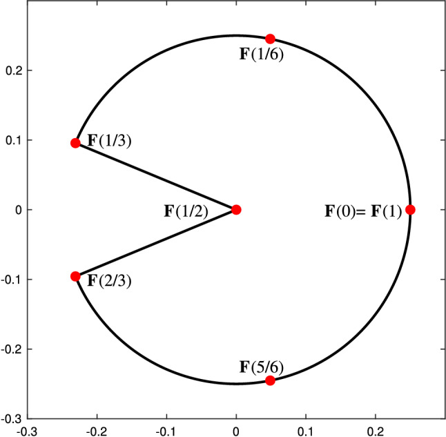
Geometry and initial vertices for the experiment of Sect. 7.3.5

Fig. 46

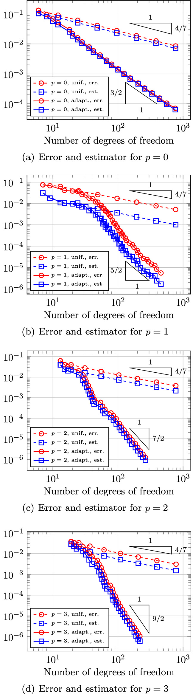
Singularity on pacman: Energy error $\Vert \varphi -{\Phi }_k{\Vert }_{\mathcal{V}}$ and estimator ${\eta }_k$ of Algorithm 10 for splines of degree p are plotted versus the number of degrees of freedom. Uniform and adaptive ($\theta =0.75$) refinement is considered

Fig. 47

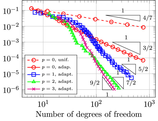
Singularity on pacman: The energy errors $\Vert \varphi -{\Phi }_k{\Vert }_{\mathcal{V}}$ of Algorithm 10 for splines of degree $p\in \{0,1,2,3\}$ are plotted versus the number of degrees of freedom. Uniform (for $p=0$) and adaptive ($\theta =0.75$ for $p\in \{0,1,2,3\}$) refinement is considered

Fig. 48

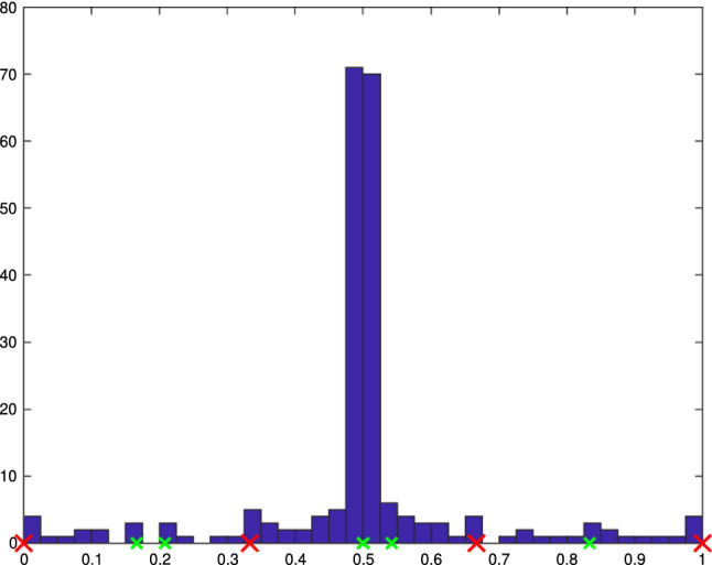
Singularity on pacman: Histogram of number of knots over the parametric domain for the knot vector $T_{29}$ generated in Algorithm 10 (with $\theta =0.75$) for splines of degree $p=3$. Knots with maximal multiplicity $p+1=4$ are marked with a red cross and knots with multiplicity 3 are marked with a green smaller cross

References

-
- AC07066955, A . Computer methods in applied mechanics and engineering. Amsterdam: Elsevier; 2017. Special issue on isogeometric analysis: progress and challenges.
- Actis M, Morin P, Pauletti MS. A new perspective on hierarchical spline spaces for adaptivity. Comput Math Appl. 2020;79(8):2276–2303. doi: 10.1016/j.camwa.2019.10.028. - DOI
- Ainsworth M, Oden JT. A posteriori error estimation in finite element analysis. New York: Wiley; 2000.
- Antolin P, Buffa A, Coradello L. A hierarchical approach to the a posteriori error estimation of isogeometric Kirchhoff plates and Kirchhoff-Love shells. Comput Methods Appl Mech Eng. 2020;363:112919. doi: 10.1016/j.cma.2020.112919. - DOI
- Antolin P, Buffa A, Martinelli M. Isogeometric analysis on V-reps: first results. Comput Methods Appl Mech Eng. 2019;355:976–1002. doi: 10.1016/j.cma.2019.07.015. - DOI
Publication types
Grants and funding
LinkOut - more resources
Full Text Sources