. 2023 Feb;531(3):390-414.
doi: 10.1002/cne.25432. Epub 2022 Nov 22.

Cortical synapses of the world's smallest mammal: An FIB/SEM study in the Etruscan shrew

Affiliations

Cortical synapses of the world's smallest mammal: An FIB/SEM study in the Etruscan shrew

Lidia Alonso-Nanclares et al. J Comp Neurol. 2023 Feb.

Abstract

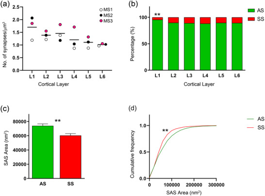
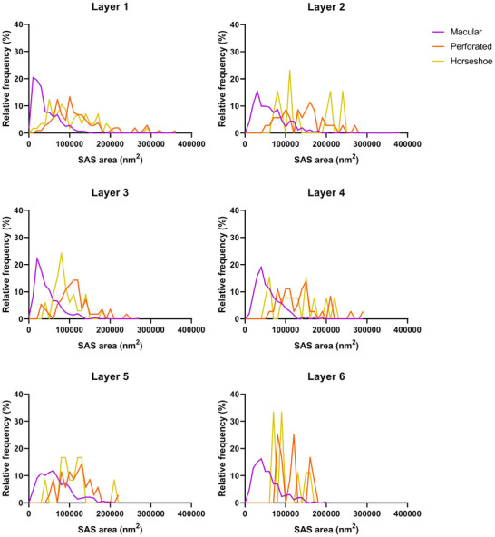
The main aim of the present study was to determine if synapses from the exceptionally small brain of the Etruscan shrew show any peculiarities compared to the much larger human brain. We analyzed the cortical synaptic density and a variety of structural characteristics of 7,239 3D reconstructed synapses, using using Focused Ion Beam/Scanning Electron Microscopy (FIB/SEM). We found that some of the general synaptic characteristics are remarkably similar to those found in the human cerebral cortex. However, the cortical volume of the human brain is about 50,000 times larger than the cortical volume of the Etruscan shrew, while the total number of cortical synapses in human is only 20,000 times the number of synapses in the shrew, and synaptic junctions are 35% smaller in the Etruscan shrew. Thus, the differences in the number and size of synapses cannot be attributed to a brain size scaling effect but rather to adaptations of synaptic circuits to particular functions.

Keywords: FIB-SEM; brain; cerebral cortex; electron microscopy; synaptic junction; ultrastructure.


Conflict of interest statement

The authors declare that they have no conflict of interest.

Figures

FIGURE 1
FIGURE 1
Correlative light‐electron microscopy study of the Etruscan shrew cerebral cortex. (a) Low power photograph of a 150 µm Nissl stained coronal vibratome section of the Etruscan shrew brain. The delimitation of cortical areas and layers is based on Naumann et al. (2012). (b) Higher magnification of the boxed area in (a), showing the laminar pattern of Som cortex (layers 1 to 6 are indicated). (c) 1 µm‐thick semithin section stained with toluidine blue. (d) Higher magnification of the boxed area in (c), showing delimitated layers based on the staining pattern. The semithin section is adjacent to the block for FIB/SEM imaging. (e) SEM image illustrating the block surface with trenches made in the neuropil (one per layer). Arrows in (d) and (e) point to the same blood vessel, showing that the exact location of the region of interest was accurately determined. Scale bar shown in (e) represents 200 µm in (a), 60 µm in (b), 105 µm in (c), 50 µm in (d) and 55 µm in (e). Cing—Cingulate Cortex; Pm—Parietal Medial Cortex; Som—Somatosensory Cortex; Ins—Insular Cortex; Pir—Piriform Cortex.
FIGURE 2
FIGURE 2
Images of neuropil in layer 3 of Etruscan shrew somatosensory cortex obtained by FIB/SEM. (a) Two synapses are indicated as examples of asymmetric (AS, green arrow) and symmetric (SS, red arrow) synapses. (b, c) Higher magnification of AS (b) and SS (c) indicated in (a). Synapse classification was based on the examination of the full sequence of serial images (see Figure 3). Scale bar in (c) represents 500 nm in (a), and 250 nm in (b) and (c).
FIGURE 3
FIGURE 3
Sequence of FIB/SEM serial images of an AS (a–h) and an SS (i–p) indicated in Figure 2. Numbers on the top right of each panel indicate the number of each section from a stack of serial sections. Synapse classification was based on the examination of full sequences of serial images, see Section 2.4 for further details. Asterisks (in d–h) indicate a spine apparatus in a postsynaptic dendritic spine head. Scale bar shown in (p) represents 500 nm in (a–p).
FIGURE 4
FIGURE 4
Screenshot of the EspINA software user interface. (a) In the main window, the sections are viewed through the xy plane (as obtained by FIB/SEM microscopy). The other two orthogonal planes, yz and xz, are also shown in adjacent windows (on the right). (b) 3D reconstructions of segmented AS (green) and SS (red). (c) Computed SAS for each reconstructed synapse (yellow). (d) Table of synaptic 3D morphometric data from AS automatically obtained by EspINA software. Scale bar in (c) represents 5 µm in (b) and (c).
FIGURE 5
FIGURE 5
Plots of the synaptic analysis of the Etruscan shrew somatosensory cortex. (a) Mean of the overall synaptic density from each layer. Different colors correspond to each analyzed animal, as denoted in the upper right‐hand corner. (b) Proportion of AS and SS per layer expressed as percentages, showing that layer 1 was different from the other layers (χ2; p < .0001). (c) Mean SAS area per synaptic type shows larger synaptic size of AS compared to SS (MW, p = .0015). (d) Cumulative frequency distribution graph of SAS area illustrating that small SS (red) were more frequent (KS, p < .0001) than small AS (green). Asterisks indicate statistically significant differences.
FIGURE 6
FIGURE 6
Analysis of the 3D synaptic spatial distribution in somatosensory cortex from the Etruscan shrew. Red dashed traces correspond to a theoretical homogeneous Poisson process for each function (F, G, K). The black continuous traces correspond to the experimentally observed function in the sample. The shaded areas represent the envelopes of values calculated from a set of 99 simulations. Plots show a distribution which fits into a Poisson function, but the experimental function from layer 3 for the G‐function is partially out of the envelope. Plots obtained in layer 1 and layer 3 from animal MS1.
FIGURE 7
FIGURE 7
Frequency histograms of SAS areas and their corresponding best‐fit probability density functions. (a, b) Frequency histograms of SAS areas in the six cortical layers are represented for AS and SS in a and b, respectively. (c, d) Frequency histograms (white bars) and best‐fit distributions of the theoretical probability synaptic density functions (magenta traces) have been represented. The best‐fit probability functions were log‐normal distributions. Curve fitting was always better for AS (c) than for SS (d), probably because of the smaller sample size of SS (Table 4). The parameters µ and σ of the log‐normal curves are shown in Table 4.
FIGURE 8
FIGURE 8
Study of the different synaptic shapes. (a) Schematic representation of the synaptic shapes: macular synapses, with a continuous disk‐shaped PSD; perforated synapses, with holes in the PSD; horseshoe‐shaped, with a tortuous perimeter with an indentation in the PSD. (b) Proportions of the different synaptic shapes of AS per cortical layer. Significantly fewer macular AS were found in layer 1, compared to the rest of the layers (χ2, p <  .0001).
FIGURE 9
FIGURE 9
Frequency distribution plots of SAS area of AS per cortical layer. Different colors correspond to each synaptic shape, as denoted in the key. Statistical comparisons showed differences in the frequency distribution of the SAS area of macular synapses compared to perforated and horseshoe‐shaped synapses (KS, p < .0001).
FIGURE 10
FIGURE 10
3D reconstruction of a dendritic segment from FIB/SEM serial images. (a–f) Images 121, 129, 134, 136, 140, and 155 from a stack of serial sections obtained with FIB/SEM, showing a dendritic segment partially reconstructed (in purple). An asymmetric synapse (green arrow) on a dendritic spine, and a symmetric synapse (red arrow) on the shaft are indicated. (g–h) 3D reconstructions of the same dendritic segment are displayed, after rotation about the major dendritic axis. The dendritic spine is shown establishing an asymmetric synapse (green)—and one symmetric synapse (red) on the shaft is also visible. Note that the shape of the asymmetric synapse can be identified as perforated (h). Scale bar (in h) indicates 1400 nm in a–f and 700 nm in g, h.
FIGURE 11
FIGURE 11
Proportions of postsynaptic targets—dendritic spines and shafts—of AS per cortical layer. AS show a significant preference for spines in all layers (χ2; p < .0001). Layers 4, 5 and 6 displayed a greater proportion of AS on spines than layers 1, 2, and 3 (χ2; p < .0001).

Similar articles

Cited by

References

    1. Alonso‐Nanclares, L. , Gonzalez‐Soriano, J. , Rodriguez, J. R. , & DeFelipe, J. (2008). Gender differences in human cortical synaptic density. Proceedings of the National Academy of Sciences, 105(38), 14615–14619. 10.1073/pnas.0803652105 - DOI - PMC - PubMed
    1. Amunts, K. , & Zilles, K. (2015). Architectonic mapping of the human brain beyond Brodmann. Neuron, 88(6), 1086–1107. 10.1016/j.neuron.2015.12.001 - DOI - PubMed
    1. Anjum, F. , Turni, H. , Mulder, P. G. H. , van der Burg, J. , & Brecht, M. (2006). Tactile guidance of prey capture in Etruscan shrews. Proceedings of the National Academy of Sciences, 103(44), 16544–16549. 10.1073/pnas.0605573103 - DOI - PMC - PubMed
    1. Anton‐Sanchez, L. , Bielza, C. , Merchán‐Pérez, A. , Rodríguez, J.‐R. , DeFelipe, J. , & Larrañaga, P. (2014). Three‐dimensional distribution of cortical synapses: A replicated point pattern‐based analysis. Frontiers in Neuroanatomy, 8. 10.3389/fnana.2014.00085 - DOI - PMC - PubMed
    1. Ascoli, G. A. , Alonso‐Nanclares, L. , Anderson, S. A. , Barrionuevo, G. , Benavides‐Piccione, R. , Burkhalter, A. , Buzsáki, G. , Cauli, B. , Defelipe, J. , Fairén, A. , Feldmeyer, D. , Fishell, G. , Fregnac, Y. , Freund, T. F. , Gardner, D. , Gardner, E. P. , Goldberg, J. H. , Helmstaedter, M. , Hestrin, S. , … Yuste, R. (2008). Petilla terminology: nomenclature of features of GABAergic interneurons of the cerebral cortex. Nature Reviews Neuroscience, 9, 557–568. 10.1038/nrn2402 - DOI - PMC - PubMed

Publication types