. 2023 Jan;613(7944):543-549.
doi: 10.1038/s41586-022-05471-w. Epub 2022 Nov 23.

Structured cerebellar connectivity supports resilient pattern separation

Affiliations

Structured cerebellar connectivity supports resilient pattern separation

Tri M Nguyen et al. Nature. 2023 Jan.

Erratum in

Abstract

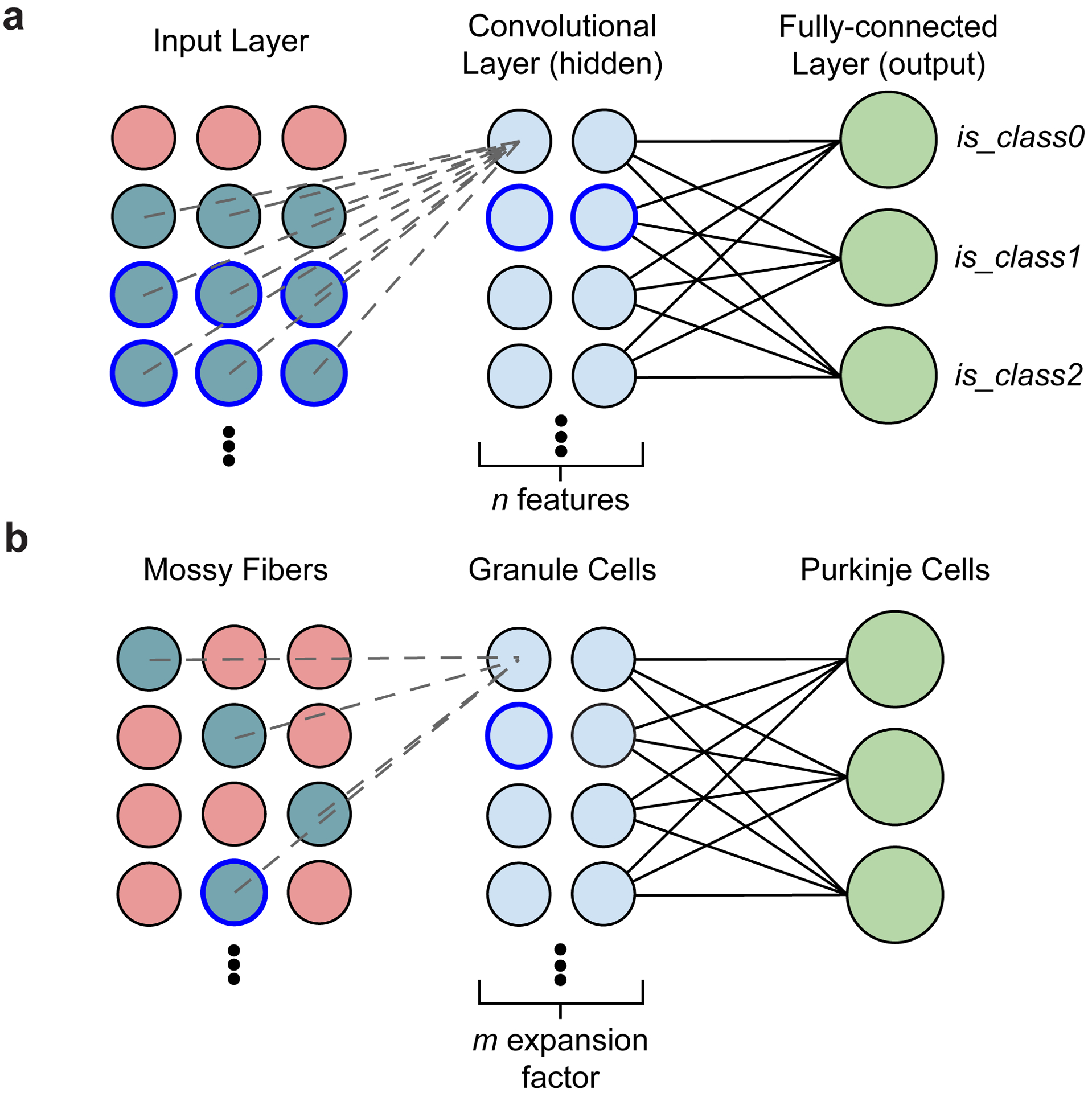
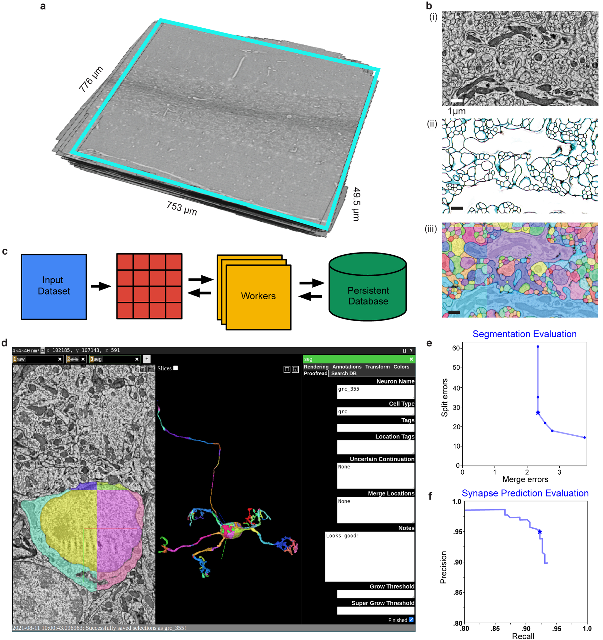
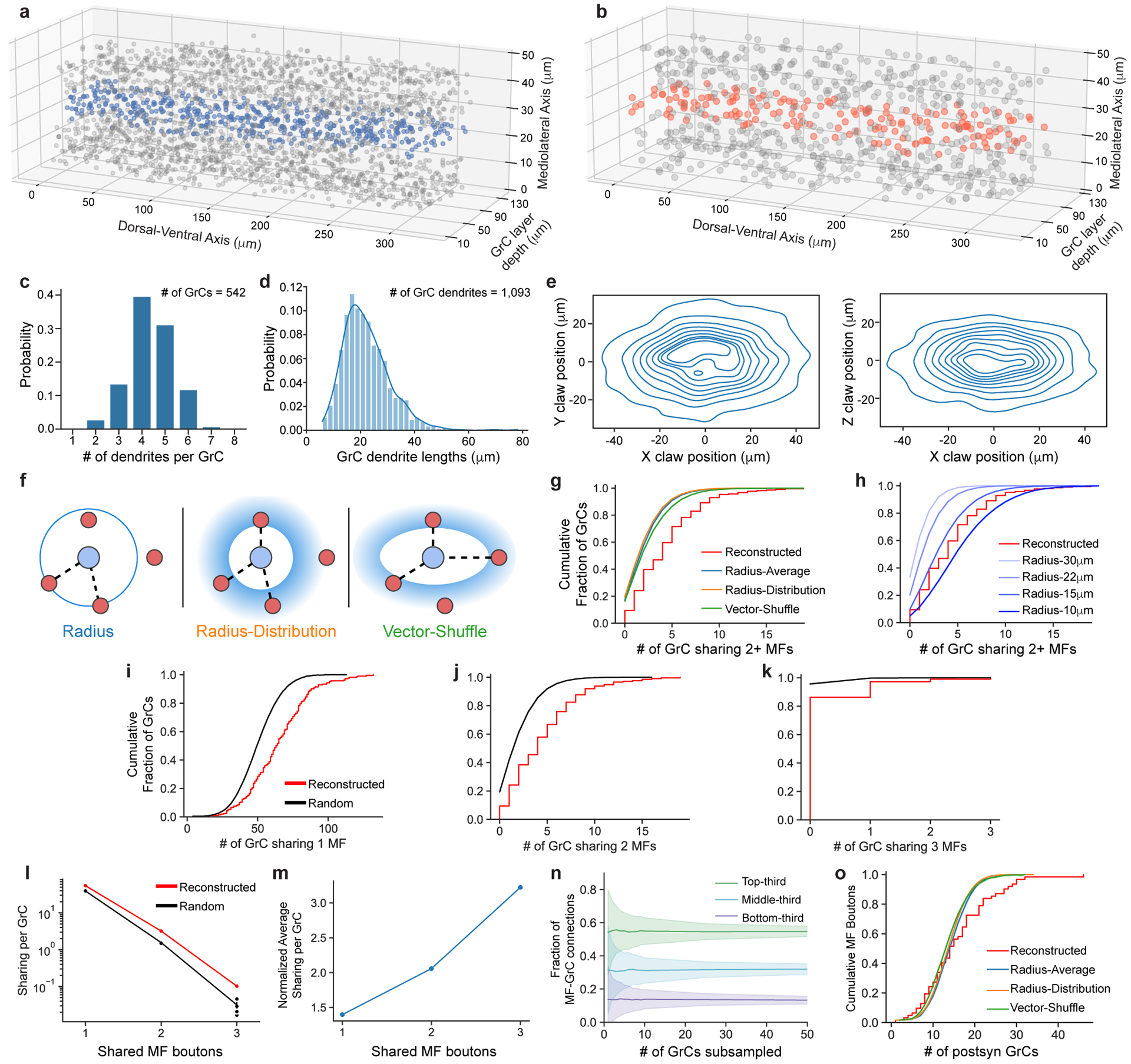
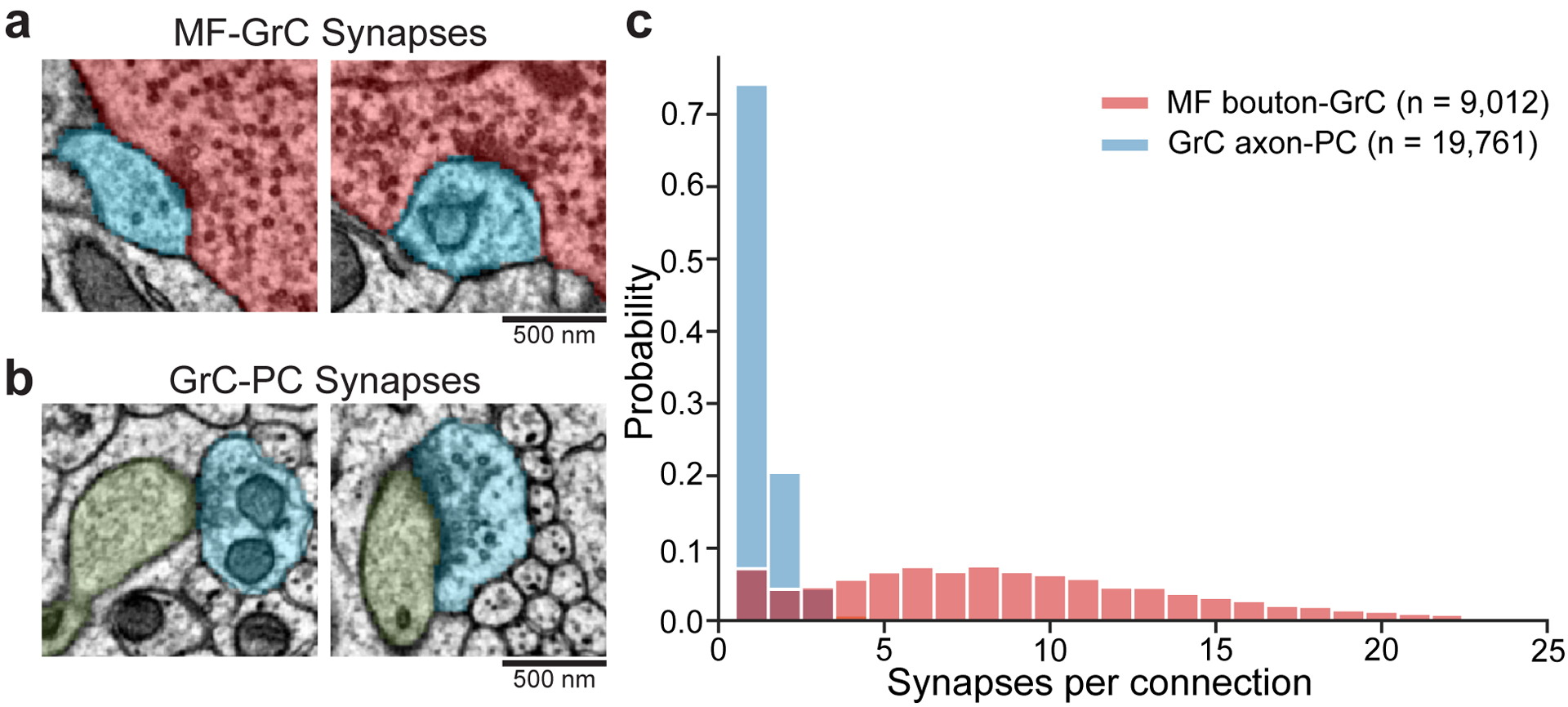
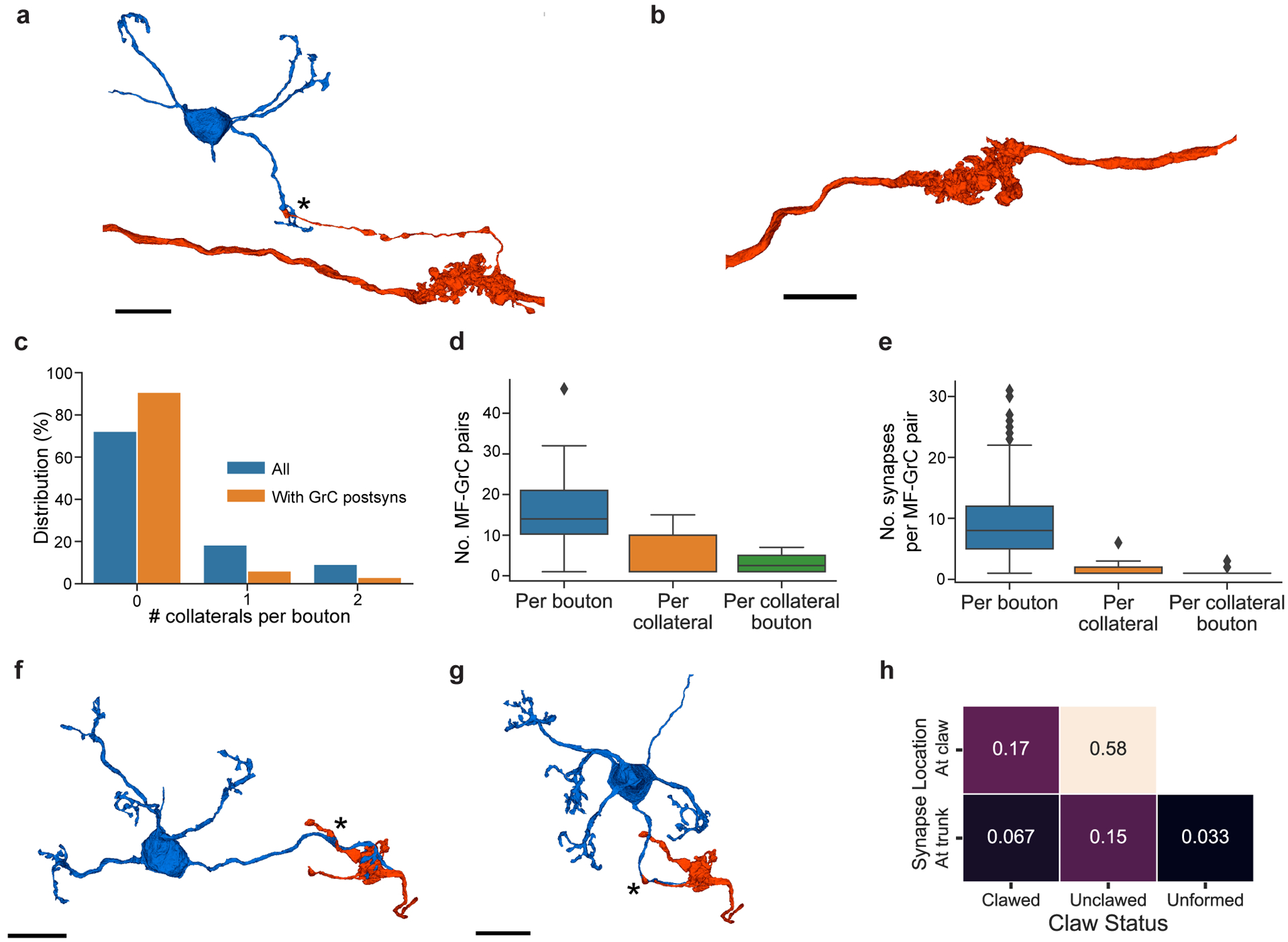
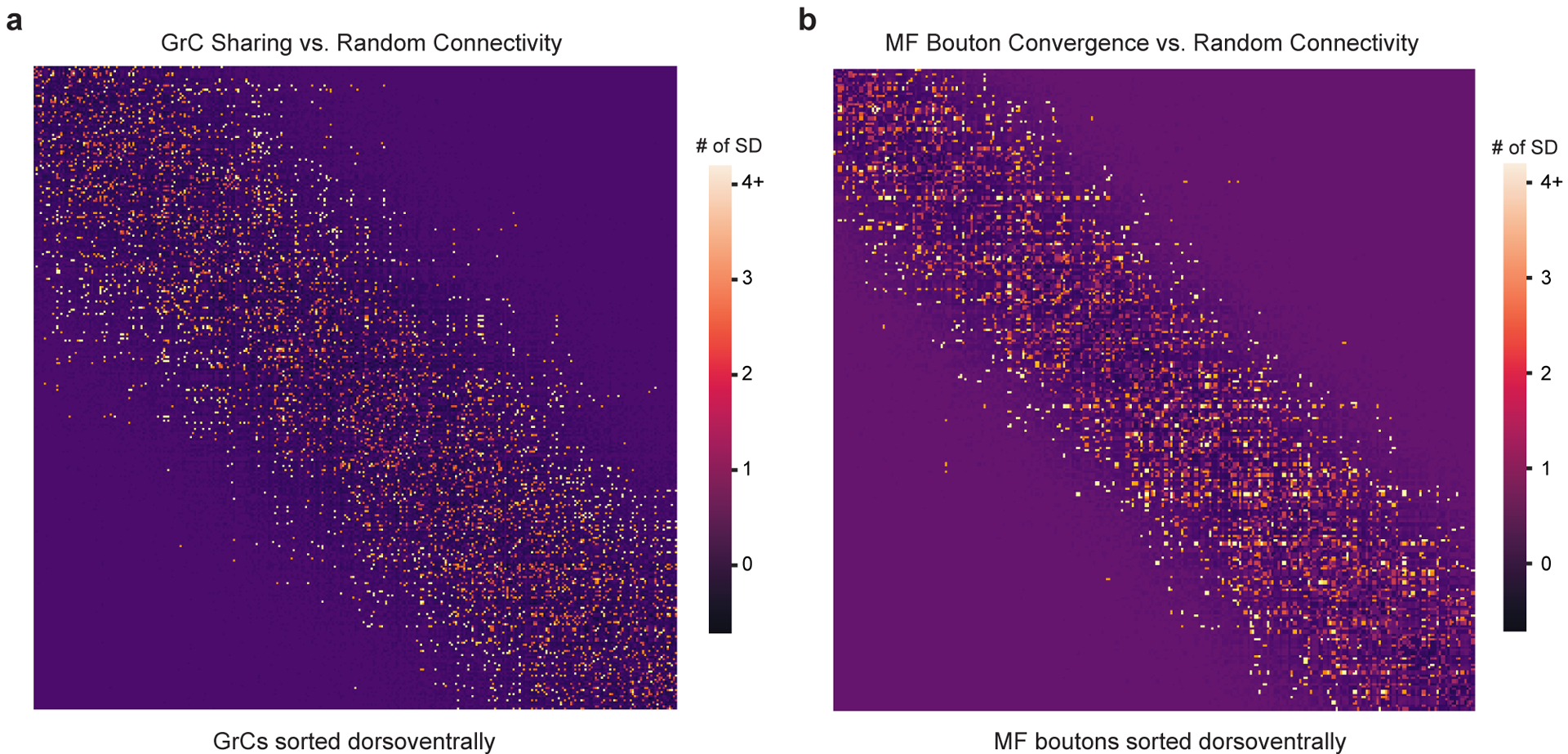
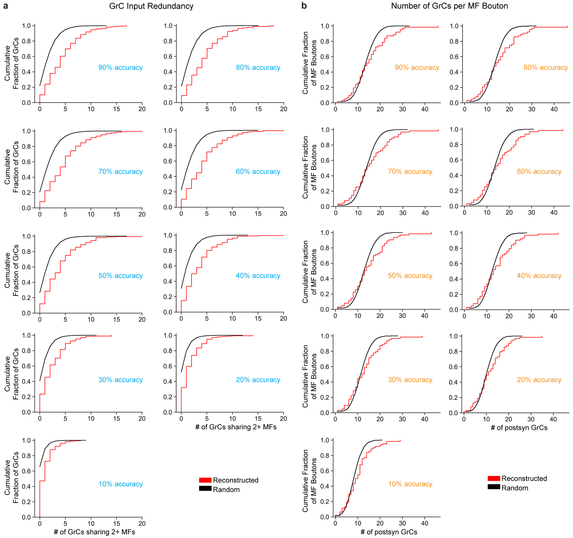
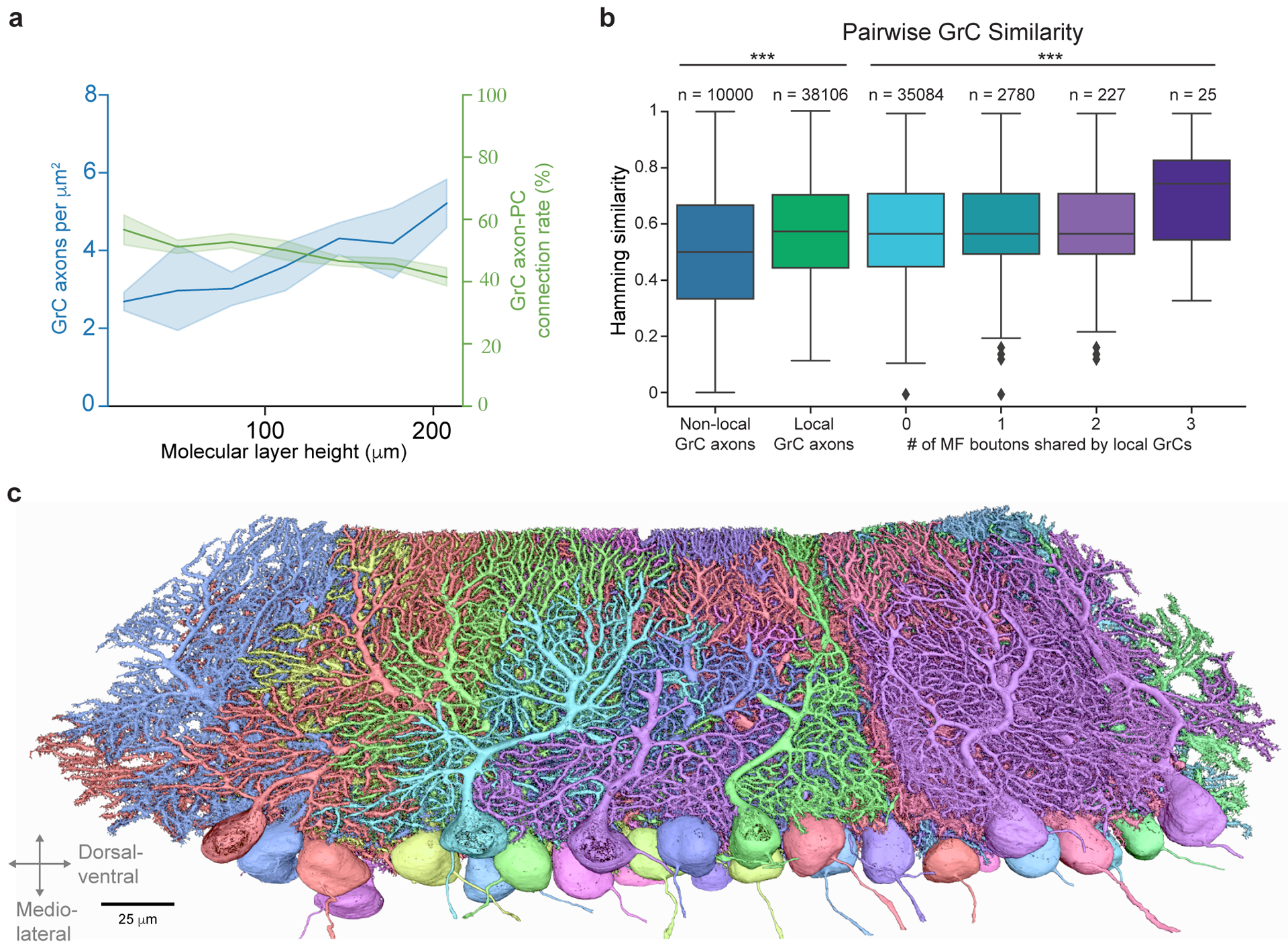
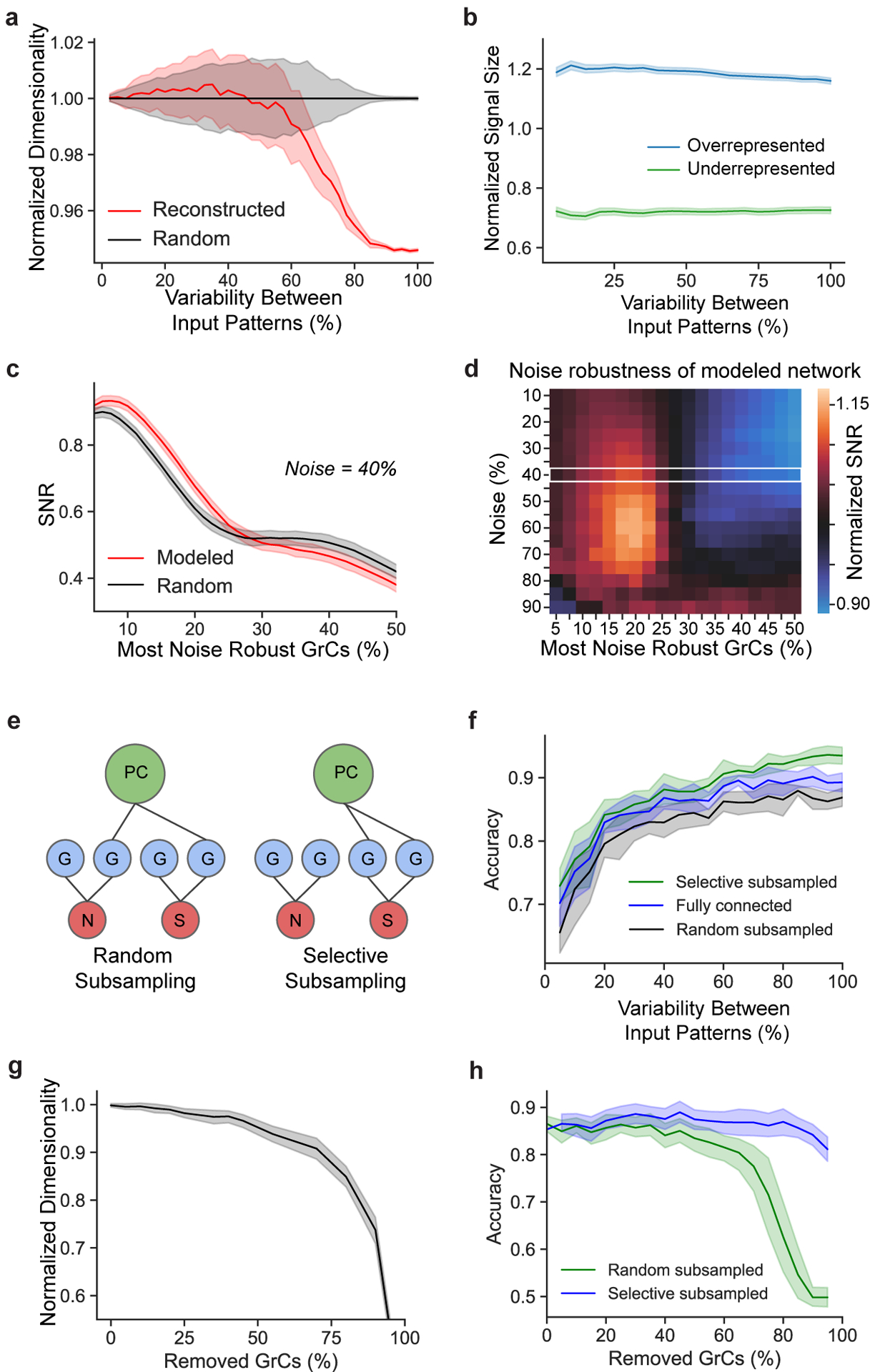
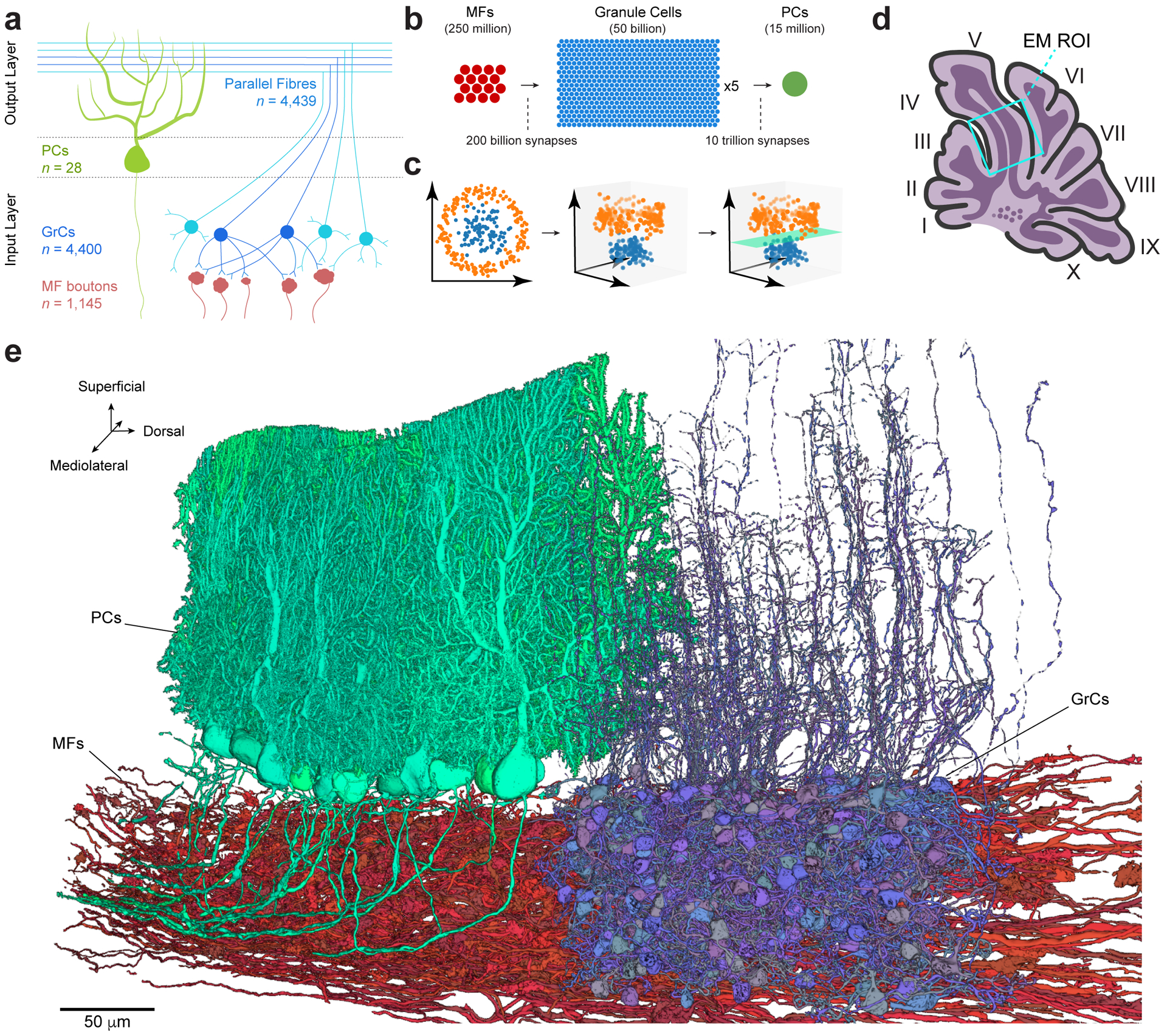
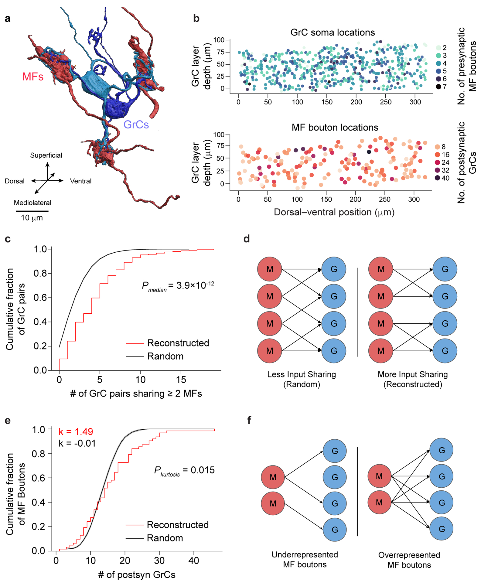
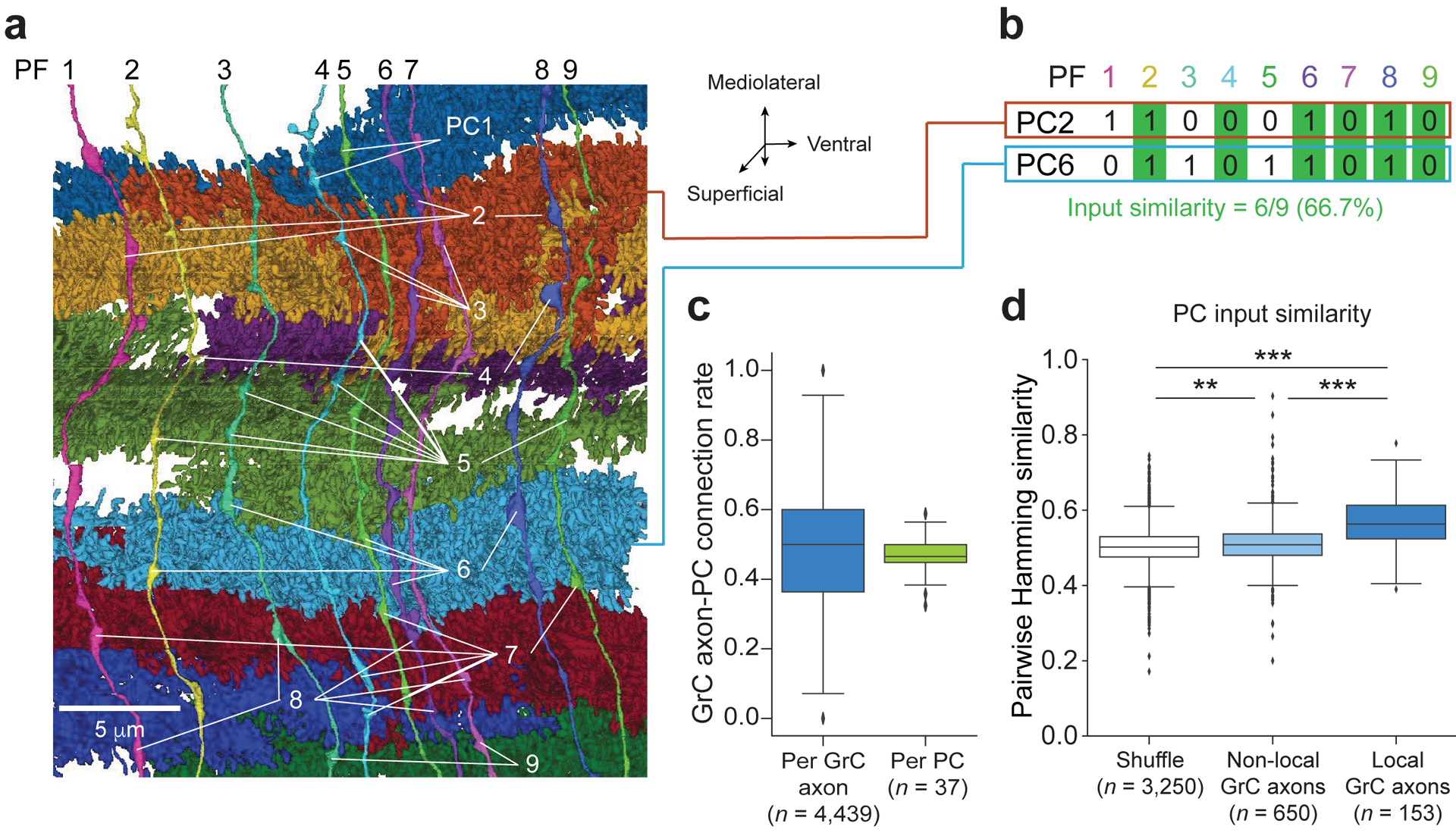
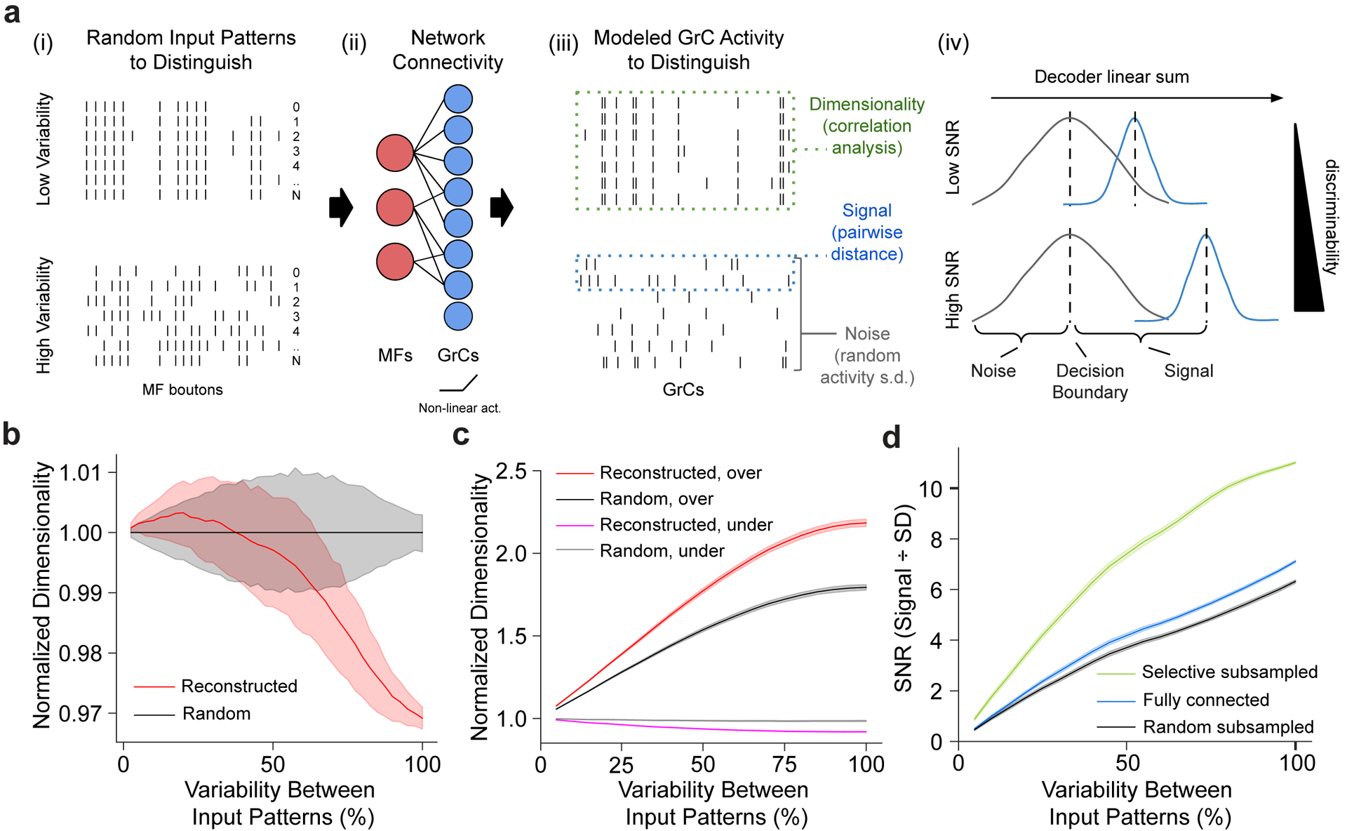
The cerebellum is thought to help detect and correct errors between intended and executed commands1,2 and is critical for social behaviours, cognition and emotion3-6. Computations for motor control must be performed quickly to correct errors in real time and should be sensitive to small differences between patterns for fine error correction while being resilient to noise7. Influential theories of cerebellar information processing have largely assumed random network connectivity, which increases the encoding capacity of the network's first layer8-13. However, maximizing encoding capacity reduces the resilience to noise7. To understand how neuronal circuits address this fundamental trade-off, we mapped the feedforward connectivity in the mouse cerebellar cortex using automated large-scale transmission electron microscopy and convolutional neural network-based image segmentation. We found that both the input and output layers of the circuit exhibit redundant and selective connectivity motifs, which contrast with prevailing models. Numerical simulations suggest that these redundant, non-random connectivity motifs increase the resilience to noise at a negligible cost to the overall encoding capacity. This work reveals how neuronal network structure can support a trade-off between encoding capacity and redundancy, unveiling principles of biological network architecture with implications for the design of artificial neural networks.


Conflict of interest statement

Competing interests

W.C.A.L. and D.G.C.H. declare the following competing interest: Harvard University filed a patent application regarding GridTape (WO2017184621A1) on behalf of the inventors including W.C.A.L. and D.G.C.H., and negotiated licensing agreements with interested partners.

Figures

Extended Data Figure 1.
Extended Data Figure 1.. Similarity between a convolutional neural network and the cerebellar feedforward network.
a, Diagram of a simple convolutional neural network with one convolutional layer (input→hidden) and one fully connected layer (hidden→output). The input (left) is made up of a single-channel 2D grid of neurons. The convolutional layer (middle) is made up of neurons each sampling a small local grid of the input (e.g., nine inputs when a 3×3 filter is used, cyan colored circles). This is notably different from a multi-layer perceptron network where the input and the hidden layer are fully connected - the convolution allows an increase in features while decreasing computational cost. Due to the small field of view of each convolutional layer neuron, adjacent neurons share a significant amount of inputs with each other. To increase capacity of the hidden layer, the convolutional neurons can be replicated by n times (typically parameterized as n features). Finally, the output neurons (right) are fully connected with neurons in the preceding convolutional layer. For a classification network, each label (class) is associated with a single binary output neuron for both training and inference. b, Diagram of the cerebellar feedforward network. Mossy fibers (MFs; left) can be considered a 2D grid of sensory and afferent command inputs typically of mixed modalities,. Granule cells (GrCs; middle) sample only ~4 MF inputs each. The total number of GrCs is estimated to be hundreds of times more than the number of MFs (Fig. 1b), represented by an expansion factor m. Finally, Purkinje cells (PCs; right) - output neurons of the cerebellar cortex - receive input from tens to hundreds of thousands of GrC axons that pass by PC dendrites.
Extended Data Figure 2.
Extended Data Figure 2.. Automated segmentation and synapse prediction
a, Serial-section electron microscopy (EM) dataset from lobule V from the cyan boxed region in Fig. 1d. b, The 3D reconstruction segmentation pipeline. (i) EM image data, (ii) boundary affinities, and (iii) automated segmentation output. c, Parallelized volume processing using Daisy. The input dataset is divided into small blocks, on which multiple workers can dynamically query and work. Block completion status and output data are efficiently stored into a persistent database or on disk directly from the workers without going through the centralized scheduler process. d, Example view of targeted neuron reconstruction using merge-deferred segmentation (MD-Seg). Neurons are first segmented as small blocks, and inter-block merge decisions are deferred to proofreaders. This is illustrated by the different colored segments of the displayed neuron. The user interface is based on Neuroglancer, modified to provide the segment “grow” functionality, and to integrate an interface to the database keeping track of neuron name, cell type, completion status, notes, and which agglomeration threshold to use for “growing”, as well as searching for neurons based on different criteria and recoloring segments of a single neuron to a single color (“Search DB” and “Color” tabs, not shown). e, Automated segmentation evaluation; plot points denote agglomeration thresholds. Average number of merge and split errors of (n = 9) 6 μm test volumes. We used a threshold (star) with 2.33 merges and 27 splits per 6 μm for proofreading. f, Automated synapse prediction evaluation; plot points denote connected component thresholds. Precision and recall curve for the synapse inference network. We achieved high synapse prediction accuracy with precision: 95.4% and recall: 92.2%, and an f-score: 93.8% (star)..
Extended Data Figure 3.
Extended Data Figure 3.. MF→GrC wiring, convergence, and null models.
a,b, 3D plot of the locations of GrC somas and centers of MF boutons reconstructed in the 320 × 80 × 50 μm subvolume. Blue and orange dots indicate the GrCs and MF boutons respectively in the center 10 μm in the mediolateral axis, as plotted in Fig. 2b. c, Distribution of the number of dendrites per GrC (n = 542). d, Distribution of GrC dendrite lengths (n = 1093). e, Anisotropic positioning of MF bouton→GrC inputs (claws), showing elongated distribution in the dorsal-ventral axis (X) relative to both anterior-posterior (Y) and medio-lateral (Z) axes. Contour lines represent 10% intervals in the distribution. f, MF→GrC random models used for comparison with the reconstructed connectivity. (Methods). g, Similar to Fig. 2c, but with random models from f added. h, Similar to g, but with Radius models of different dendrite lengths. i, Cumulative distribution of MF bouton input redundancy counting the number of GrC pairs sharing 1 MF bouton (similar to Fig. 2c). j, Similar to i, but for 2 MF boutons. k, Similar to i, but for 3 MF boutons. l, Average number of GrC pairs sharing 1, 2, or 3 common MF bouton inputs, comparing reconstructed against the Radius random connectivity model described in d. m, Average sharing of GrCs in the reconstructed network as in l, but normalized to random networks. n, Average fractional distribution of inputs to GrCs from different MF bouton types (categorized as the top-third, middle-third, and bottom third most connected boutons) as a function of GrC sampling size. GrCs were randomly subsampled to produce input composition distributions, with error shadings representing SD. o, Same as Fig. 2e, but with random models from f added.
Extended Data Figure 4.
Extended Data Figure 4.. MF→GrC and GrC→PC synaptic connectivity.
a, Example EM micrographs of MF (red) to GrC (blue) synapses. b, Example EM micrographs of GrC (blue) to PC (green) synapses. c, Distributions of the number of synapses per connection of the two synapse types. We analyzed (n = 9012) MF→GrC and (n = 19761) GrC→PC synapses in one volumetric EM dataset from one animal. The median of MF→GrC is nine synapses, while GrC→PC is one. Over 97% of GrC→PC unitary connections have 1 to 2 synapses, though instances of 3 to 6 synapses per connection, while rare, do occur.
Extended Data Figure 5.
Extended Data Figure 5.. MF collateral axons connectivity to GrCs.
a, 3D rendering of a MF (red) bouton, with an axon collateral making synapses onto a GrC (blue) dendrite near a claw. Asterisks denote the location of synapses. b, Rendering of a MF bouton with no axon collaterals. c, Distribution of number of collaterals per MF bouton (n = 63); a MF bouton can have multiple axon collaterals, and each collateral may or may not make synapses onto GrCs. d, Box plot (25th, 50th and 75th percentiles with whiskers extended to points within 1.5 IQRs) of the number of MF-GrC connections: per MF bouton (n = 63), per axon collateral (n = 8), and per each bouton in a collateral (n = 16). e, Box plot of the number of synapses in each MF-GrC connection: per MF bouton (n = 978), per collateral (n = 28), and per bouton in collateral axons (n = 51). Due to the low frequency of axon collaterals, GrC targets, and the number of synapses per GrC target, it is unlikely that MF axon collaterals to GrCs represent a major route of signal propagation. f, Example of an axon collateral making synapses to a GrC on the trunk, and with more synapses formed on the claw. g, Example of a connection on the trunk of the dendrite, with no claw. h, Joint probability distribution of the synapse location of MF axon collaterals onto GrCs (on claw vs. trunk) and whether or not the dendrite made a claw onto the same MF bouton, or did not have claws (unformed claws). These examples of MF axon collateral connections to GrCs could represent different states of MF→GrC rewiring, supporting the hypothesis that MF→GrC wiring adapts to changing MF input representation,. Scale bars are 10 μm.
Extended Data Figure 6.
Extended Data Figure 6.. MF→GrC oversharing and convergence vs null models.
a, GrC input sharing relative to random connectivity. The matrix shows the degree of input sharing between GrCs (centermost n = 550, sorted by soma position dorsoventrally). The color scale for each cell in the matrix uses the z-score (reconstructed # of sharing minus random mean divided by the SD). b, MF bouton output convergence relative to random connectivity. The matrix shows the degree of output convergence between MF boutons (centermost n = 234, sorted by soma position dorsoventrally). The color scale uses the z-score as in a.
Extended Data Figure 7.
Extended Data Figure 7.. Synapse prediction sensitivity analysis.
a, Cumulative distributions of MF bouton input redundancy as in Fig. 2c but across synapse prediction accuracies ranging from 90% to 10%. We artificially added false positives (FPs) and false negatives (FNs) to the network (Extended Data Fig. 2f) to achieve different accuracies (Methods). b, Cumulative distribution of postsynaptic GrCs per MF bouton as in Fig. 2e but across synapse prediction accuracies. As shown in a and b, we found that the results were consistent across models and only changed substantially when the FP/FN rates increased past 60%. We propose two reasons our results are robust across model prediction accuracies. First, MF-GrC connections are typically composed of multiple synapses (10 on average, Extended Data Fig. 4c). Since we used at least 3 synapses as a threshold for determining connectivity, even with significant missing, undetected synapses (eg. 50%), the remaining synapses are still reliable to reflect binary connectivity. Second, random and spurious false positive predictions are unlikely to coincide to cross the 3-synapse threshold. One interesting implication is that strongly selective features do not require perfect synapse prediction. This is consistent with connectomes in Drosophila where synapse prediction accuracy is ~60% and that connections are typically consist of multiple synapses which means that even with significant missing, undetected synapses (eg. 50%), the remaining synapses are sufficiently reliable to indicate connectivity.
Extended Data Figure 8.
Extended Data Figure 8.. GrC→PC wiring and similarity of inputs to PCs.
a, Plot of density GrC axons and GrCPC connectivity rate as a function of height in the molecular layer between the pial surface and PC layer. Across molecular heights, the average axon density is 3.73 ± 1.23 per μm (mean ± SD), and the average connection rate is 49.12 ± 4.39% (mean ± SD). Using these numbers and the average area of PC dendrites, we calculated ~125,000 GrC axons pass through the dendritic arbor of each reconstructed PC. At an average connectivity rate of 49%, only about 60,000 GrC axons were connected to each PC, 3–5× less than typically assumed in models of the cerebellar cortex,,. b, Box plot (25th, 50th and 75th percentiles with whiskers extended to points within 1.5 IQRs) of pairwise Hamming similarity between PC postsynaptic targets of non-local GrC axons, and local GrC axons with different numbers of shared MF bouton inputs. Across local GrCs sharing 0, 1, 2, and 3 MF boutons, Hamming similarity means = p = 0.0001137, Kruskal-Wallis H-test. 0-shared vs 1-shared p = 0.0132, 0-shared vs 3-shared p = 0.00797, 1-shared vs 3-shared p = 0.0186, 2-shared vs 3-shared p = 0.0309, other pairings p > 0.05, Dunn’s post hoc tests, Bonferroni corrected for multiple comparisons. c, 3D rendering of EM reconstructed PCs arbitrarily colored.
Extended Data Figure 9.
Extended Data Figure 9.. MF-GrC-PC simulations
a, Normalized dimensionality of GrCs as a function of input variability using a continuous model of spike frequency. Noise was modeled as the degree of variation of spiking frequency across all MF inputs (Methods). b, Modeled learned signal size (Methods) as a function of variability between MF input patterns, comparing pattern separation performance between overrepresented (top-third most connected) and underrepresented (bottom-third) MF boutons. Signal size from the reconstructed network is normalized by the random connectivity model for each population separately. c-d, SNR analyses of modeled MF-GrC networks, measuring noise robustness with (Modeled) or without (Random) redundant oversharing of MF inputs (Fig. 2c,d). SNR was computed across GrC subpopulations ranked by robustness (Methods) at a 40% noise level in c, and across GrC subpopulations and noise levels in d (normalized to SNRs of the “random” model at each noise level and subpopulation). The white box in d denotes the noise level shown in c. Redundant oversharing helps PCs learn more reliably by encoding the most robust signals in a subset of more correlated GrCs. e, Binary GrC→PC selective subsampling increases SNR. Left: PCs (green) randomly subsample GrCs (blue) with MF (red) inputs containing signal (S) or noise (N). Right: PCs connect to GrCs encoding signal-relevant MFs, leading to a higher SNR (Fig. 4d). f, Prediction accuracy of a linear neural network trained on output patterns of the GrCs as a function of MF input variability, comparing performance of MF-GrC networks between models that were fully connected, randomly subsampled with 50% connectivity, and selective subsampled with 50% connectivity, all as a function of MF input variability. g, Dimensionality of the GrC population as a function of the percentage of GrCs randomly removed, normalized to the dimensionality with 100% of the population. h, Prediction accuracy as in f comparing performance of MF-GrC networks between randomly and selectively subsampled models as a function of a percentage of randomly removed GrCs.
Figure 1.
Figure 1.. Reconstruction of feedforward circuitry in the cerebellar cortex using large-scale electron microscopy.
a, Schematic depicting wiring of feedforward neurons in the cerebellar cortex. Granule cells (GrCs, blue circles) sample mossy fiber (MF) boutons (red) and project their axons into the molecular layer where they bifurcate to form parallel fibers. GrC axons make synaptic contacts onto Purkinje cells (PCs, green), which are the sole output of the cerebellar cortex. The number (n) of reconstructed objects (MF boutons and parallel fibers) or cells with cell bodies (GrCs and PCs) in our dataset is shown. b, Expansion and convergence of the cerebellar cortex feedforward network. The number of circles is proportional to the number of neurons in the estimated global population. At the local circuit scale, however, divergence of single MF boutons to GrCs is less (ratio ~1:3), and convergence of GrCs to PCs is higher (ratio 50,000–200,000:1). c, Illustrative data showing how two input representations in 2D (left) once projected into 3D (middle) can be linearly separated (right, green plane). Marr & Albus, hypothesize that the MF→GrC dimensionality expansion supports pattern separation and the GrC→PC convergence performs pattern association. d, Schematic of a parasagittal section through the vermis of mouse cerebellum with the location of the EM dataset (Extended Data Fig. 2a) outlined (cyan box). e, 3D rendering of representative EM reconstructions of PCs (green), GrCs (blue) and MFs (red). Non-overlapping GrCs and PCs were rendered for clarity.
Figure 2.
Figure 2.. EM reconstructions reveal GrCs redundantly sample MF boutons.
a, 3D rendering of two GrCs (blue) sharing three common MF bouton inputs (red). b, Locations of GrCs (top, n = 4,400, color coded to show the number of dendrites) and MF boutons (bottom, n = 1,145, color coded to show the number of postsynaptic GrCs per bouton). Only neurons in the center 10 μm in the mediolateral axis are plotted for clarity. Within a 320 × 80 × 50 μm subvolume, there are 2,397 GrCs and 784 MF boutons, giving a density of 1,870,000 GrCs and 612,000 MF boutons per mm and a ratio of 3.06 GrCs per MF bouton. c, Cumulative distribution of MF bouton input redundancy, counting the number of GrC pairs sharing at least 2 MF boutons for each GrC. To minimize edge-effects, only the centermost GrCs (n = 211, Methods) are included in this analysis. GrCs in the reconstructed network (red line) share significantly more MF boutons than connectomically-constrained random models (Radius model Extended Data Figure 3, black line; p = 3.94 × 10⁻¹², two-sided Wilcoxon rank-sum test, Methods). Here, and throughout the figures shaded regions represent the bootstrapped 95% confidence interval around data mean unless otherwise stated. d, Illustration of redundant sampling in c showing pairs of GrCs sharing 2 common MF inputs (right) vs sharing 1 common MF input (left). e, Cumulative distribution of postsynaptic GrCs per MF bouton. The reconstructed distribution (red line) is compared with a random model (black line, as in c). To minimize edge effects, only connections from the centermost MF boutons are counted (n = 62). Kurtosis (k), a unitless measure of amount of distribution in the tails, is significantly higher in the reconstructed network than the random model suggesting over- and under-sampling of MF boutons by GrCs (p = 0.0146, n = 62, two-sided Permutation test, Methods). f, Selective subsampling of MF boutons by the GrCs in e creates underrepresented and overrepresented subpopulations.
Figure 3.
Figure 3.. GrC input selectivity predicts PC subnetworks.
a, 3D rendering of nine GrC axons, nine PCs, and the locations of synapses (white lines) connecting them. Note, unlabeled axonal varicosities are presynaptic to non-PC neurons (e.g., molecular layer interneurons). b, Calculation of Hamming similarity as a pairwise metric to compare the similarity of two binary patterns. The example compares the postsynaptic connectivity pattern between two PCs from different parallel fibers (PFs) where a “1” denotes a connection and a “0” denotes the lack of connection. c, Box plot (25th, 50th and 75th percentiles with whiskers extended to points within 1.5 IQRs) of the ratio of GrC→PC synapses to the total number of times a GrC axon and PC pair contact (touch) one another (Methods). Left: synapse ratio per GrC. Right: synapse ratio per PC. d, Similarity of GrC inputs between pairs of PCs with at least 30 common GrC axon contacts comparing shuffled input connectivity, non-local GrC axons, and local GrC axons. All three populations are significantly different (p = 1.25 × 10−56, Kruskal-Wallis test; p = 0.00433, shuffle vs. non-local GrC axons; p = 9.16 × 10⁻³², non-local GrC axons vs. local GrC axons; p = 4.91 × 10−61, shuffle vs. non-local GrC axons; Dunn’s post hoc tests, Bonferroni corrected for multiple comparisons).
Figure 4.
Figure 4.. Structured redundancy increases SNR of specific and small input differences.
a, Dimensionality and signal-to-noise (SNR) analysis. (i) Binary input patterns, modeled with different levels of variability. (ii) Input patterns are non-linearly transformed by the MF-GrC network to produce modeled GrC activity,. (iii) Output activity is analyzed for dimensionality (how correlated the activity matrix is), signal (how different each output pattern is from each other), and noise (SD of the linear sum of each pattern). (iv) Illustrative histogram of the linear sum of postsynaptic GrC-PC activity. Higher signal relative to noise implies better discriminability. b, Relative dimensionality of the GrC population as a function of variability between modeled MF input activity patterns (0% denotes no difference and 100% denotes uncorrelated randomized patterns) comparing the reconstructed (red) to connectomically-constrained randomly connected models (black) normalized to the random model. c, Relative dimensionality of the GrC population as a function of variability between MF input patterns, comparing overrepresented (top-third, red and black) vs underrepresented (bottom-third, magenta and gray) most connected MF boutons in the reconstructed (red and magenta) vs random (black and gray) connectivity models. Dimensionality is normalized by the underrepresented population in the random connectivity model. d, Modeled SNR (Methods) as a function of variability between input patterns, measuring separability of GrC activity between models with selective (green), no (blue), and random (black) subsampling (Extended Data Figure 9e).

References

    1. Wolpert DM, Miall RC & Kawato M Internal models in the cerebellum. Trends Cogn. Sci 2, 338–347 (1998). - PubMed
    1. Ebner TJ & Pasalar S Cerebellum predicts the future motor state. Cerebellum 7, 583–588 (2008). - PMC - PubMed
    1. Strick PL, Dum RP & Fiez JA Cerebellum and nonmotor function. Annu. Rev. Neurosci 32, 413–434 (2009). - PubMed
    1. Koziol LF et al. Consensus paper: the cerebellum’s role in movement and cognition. Cerebellum 13, 151–177 (2014). - PMC - PubMed
    1. Schmahmann JD Disorders of the cerebellum: ataxia, dysmetria of thought, and the cerebellar cognitive affective syndrome. J. Neuropsychiatry Clin. Neurosci 16, 367–378 (2004). - PubMed

Publication types