Recognition of the ligand-induced spatiotemporal residue pair pattern of β2-adrenergic receptors using 3-D residual networks trained by the time series of protein distance maps

Abstract

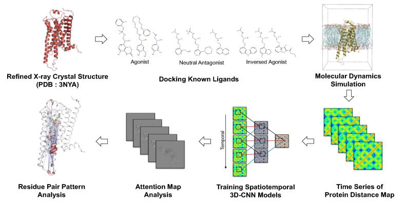
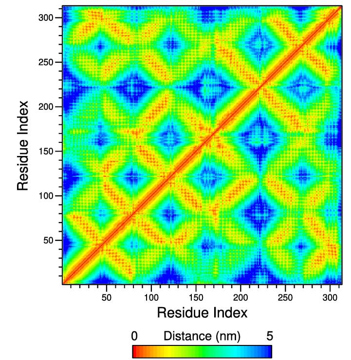
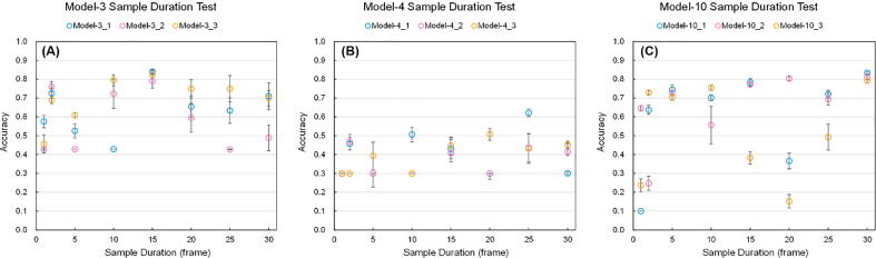
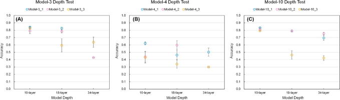
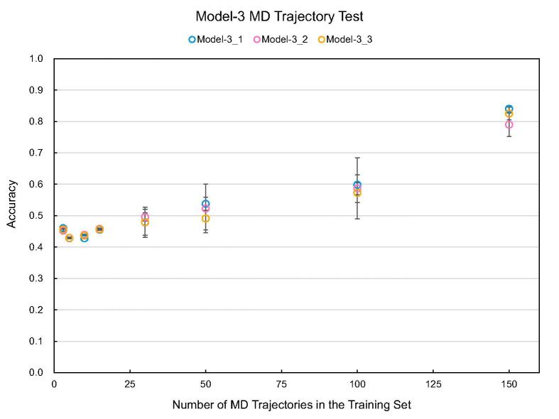
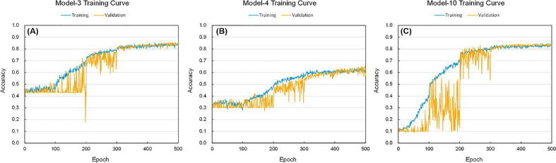
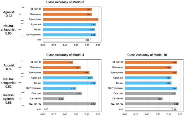
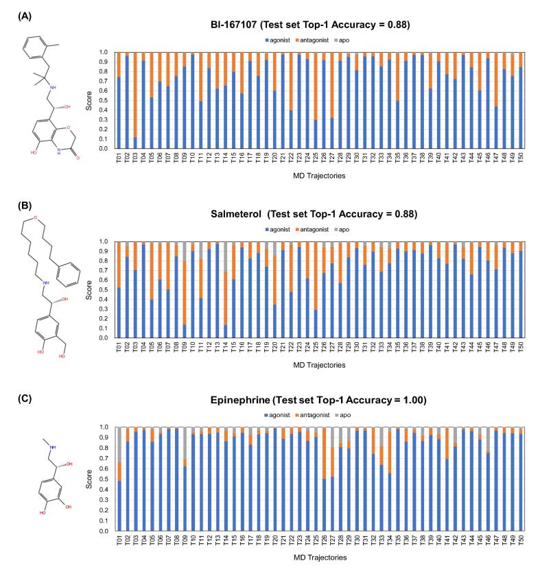
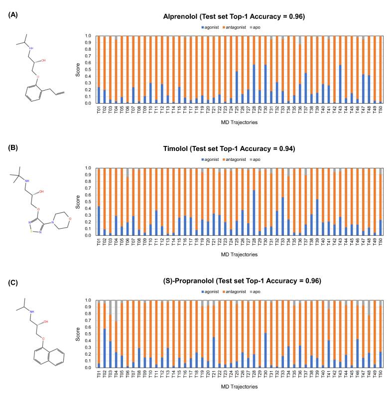
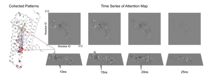
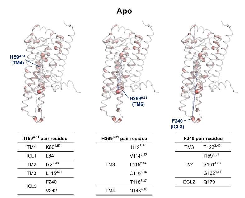
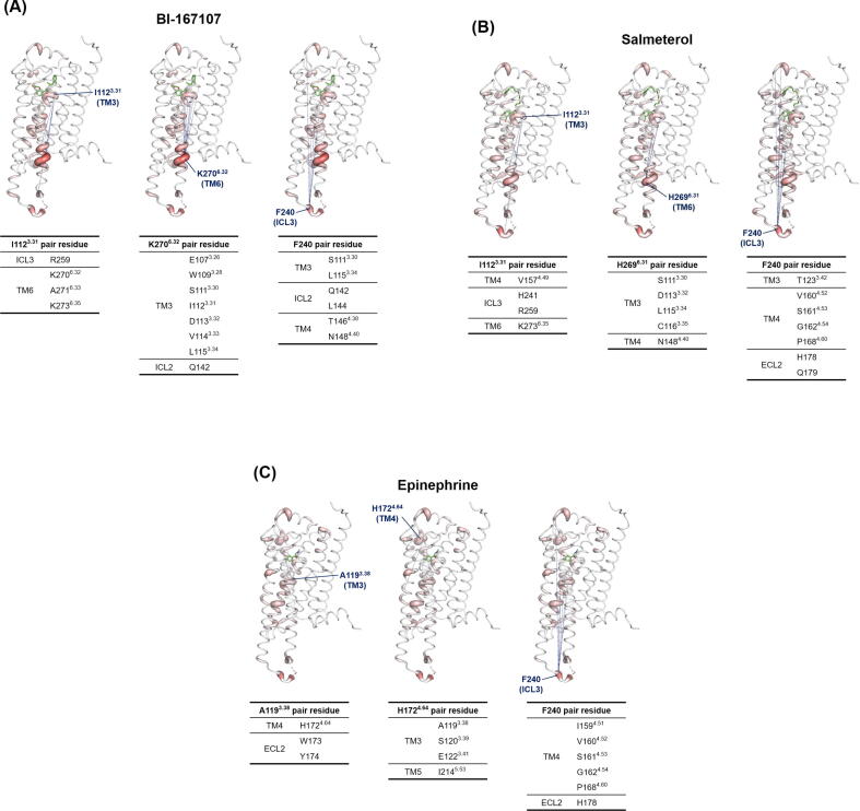
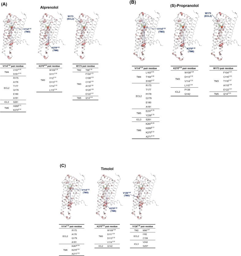
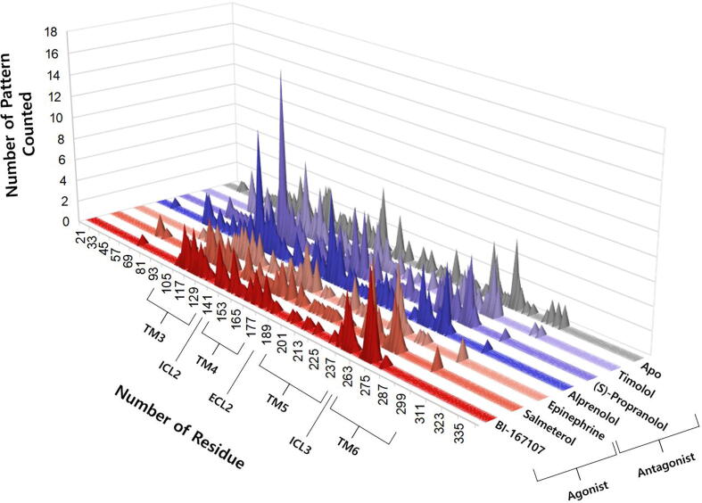
G protein-coupled receptors (GPCRs) are promising drug targets because they play a large role in physiological processes by modulating diverse signaling pathways in the human body. The GPCR-mediated signaling pathways are regulated by four types of ligands-agonists, neutral antagonists, partial agonists, and inverse agonists. Once each type of ligand is bound to the binding site, it activates, deactivates, or does not perturb signaling by shifting the conformational ensemble of GPCRs. Predicting the ligand's effect on the conformation at the binding moment could be a powerful screening tool for rational GPCR drug design. Here, we detected conformational differences by capturing the spatiotemporal residue pair pattern of the ligand-bound β2-adrenergic receptor (β2AR) using a 3-dimensional residual network, 3D-ResNets. The network was trained with the time series of protein distance maps extracted from hundreds of molecular dynamics (MD) simulation trajectories of ten β2AR-ligand complexes. The MD system was constructed with a lipid bilayer embedded in an inactive β2AR X-ray crystal structure and solvated with explicit water molecules. To train the network, three hyperparameters were tested, and it was found that the number of MD trajectories in the training set significantly affected the model's accuracy. The classification of agonists and neutral antagonists was successful, but inverse agonists were not. Between the agonists and antagonists, different residue pair patterns were spotted on the extracellular loop segment. This result demonstrates the potential application of a 3-D neural network in GPCR drug screening, as well as an analysis tool for protein functional dynamics.

Keywords: 3-D Convolution Neural Network; 3D-ResNets, 3-dimensional residual networks; Artificial Intelligence; ECL, extracellular loop; GPCR; GPCRs, G protein-coupled receptors; ICL, intracellular loop; MD, molecular dynamics; Machine Learning; Molecular Dynamics Simulation; PDM, protein distance map; Pattern Recognition; TM, TMtransmembrane helix; β2-Adrenergic Receptor; β2AR, β2-adrenergic receptor.

Fig. 1

The work flow of spatiotemporal residue pair pattern analysis.

Fig. 2

An example of a protein distance map of β2AR from the MD trajectory. The X- and Y- axis represent the residue index from 1 to 312 and each pixels represents the minimum side-chain distance between the pair of residues. The color scale below shows the color gradient from a distance of 0 to 5 nm.

Fig. 3

The averaged accuracies of the validation set for the 10-layer depth Model-3, 4, and 10 with sample durations from 1 to 30 frames shown in (A), (B), and (C). The X- and Y-axis represent the sample duration and the trained models’ accuracy, respectively. The sample duration was presented in the unit of frame in which the interval is 0.1 ns in the MD trajectory. The averaged accuracy was calculated with the last 50 epochs of the training. Each model was trained three times with the same training set with different temporal cropping points, and the results of the models are shown by blue, pick and orange lines. (For interpretation of the references to color in this figure legend, the reader is referred to the web version of this article.)

Fig. 4

The averaged accuracies of the validation set of Model-3, 4, and 10 with different number of layers, as shown in (A), (B), and (C), respectively. The X- and Y-axis represent the number of layers in the 3D-ResNets and the trained models’ accuracy, respectively. The 10-, 18-, and 34-layers represent the ResNets-10, 18 and 34 in Table 1, respectively. Each model was trained three times with the same training set with a different temporal cropping point, and the accuracies are represented in blue, pick, and orange. (For interpretation of the references to color in this figure legend, the reader is referred to the web version of this article.)

Fig. 5

The accuracies of Model-3 with different number of MD trajectories in the training set. The X- and Y-axis represent the number of MD trajectory of each ligand in the training set and model accuracy, respectively. Model-3 was trained three times with the same training set with a different temporal cropping point, and the accuracies are represented in blue, pink and orange. (For interpretation of the references to color in this figure legend, the reader is referred to the web version of this article.)

Fig. 6

Training curves of the Model-3, 4, and 10 were shown in (A), (B), and (C). The training and validation were represented in blue and orange line, respectively. The models which have the best accuracy among the sample duration test in Fig. 3 were selected. (For interpretation of the references to color in this figure legend, the reader is referred to the web version of this article.)

Fig. 7

The individual ligand and class prediction accuracy of Model-3, 4 and 10 of the Test set. In the Model-3 and 4 case, the individual ligand prediction accuracies were evaluated from the correct prediction of Top-1 accuracy of each ligand. In Model-10 case, only the individual ligand prediction was presented since the classification was performed only for the individual ligand, not for the ligand type.

Fig. 8

Evaluated scores of the three agonists, (A) BI-167107, (B) Salmeterol, and (C) Epinephrine, in the Test set-1 using the Model-3. Each agonist in the Test set-1 contains 50 MD trajectories with different initial velocity but exactly the same MD system. The scores of the agonist, neutral antagonist, and apo form were presented in blue, orange, and gray, respectively. The ligand type of the highest score in every trajectory used to determine the Top-1 accuracy. (For interpretation of the references to color in this figure legend, the reader is referred to the web version of this article.)

Fig. 9

Evaluated scores of the three neutral antagonists, (A) Alprenolol, (B) Timolol, and (C) (S)-Propranolol, in the Test set-1 using Model-3. Each neutral antagonist in the Test set-1 contains 50 MD trajectories with different initial velocity but exactly the same MD system. The scores of the agonist, neutral antagonist, and apo form are presented in blue, orange, and gray, respectively. The ligand type of the highest score in every trajectory was used to determine the Top-1 accuracy. (For interpretation of the references to color in this figure legend, the reader is referred to the web version of this article.)

Fig. 10

An example of a collected spatiotemporal pattern from the time series of the attention map obtained from a MD trajectory. In every attention map, the brightest pixel was collected and summarized. All the collected patterns were projected on the 3-dimentional structure of β2AR. The β2AR structure in tube representation on the left shows the more noticeable residue with thicker in red. Each dashed line in blue connects the pattern-associated residue pair to each other. (For interpretation of the references to color in this figure legend, the reader is referred to the web version of this article.)

Fig. 11

The three significant residues and their pairs were presented on the apo form of the β2AR structures. The thickness of the tube represents the number of pair patterns with which the residue in the position is associated. The pair residues of each significant residue are listed in the tables below the snapshots. The dashed lines in blue connects the relative residue pairs with each other. (For interpretation of the references to color in this figure legend, the reader is referred to the web version of this article.)

Fig. 12

The three significant residues and their pairs are presented on (A) the BI-167107, (B) the Salmeterol, and (C) the Epinephrine bound β2AR structures. The thickness of the tube represents the number of pair patterns with which the residue in the position is associated. The pair residues of each significant residue are listed in the tables below the snapshots. The dashed lines in blue connects the relative residue pairs with each other. (For interpretation of the references to color in this figure legend, the reader is referred to the web version of this article.)

Fig. 13

The three significant residues and their pairs are presented on (A) the Alprenolol, (B) the (S)-Propranolol, and (C) Timolol bound β2AR structures. The thickness of the tube represents the number of pair patterns with which the residue in the position is associated. The pair residues of each significant residue are listed in the tables below the snapshots. The dashed lines in blue connects the relative residue pairs with each other. (For interpretation of the references to color in this figure legend, the reader is referred to the web version of this article.)

Fig. 14

The distribution of the patterns over all residues in the seven β2AR cases. The results of the apo-form, three agonists, and three neutral antagonists bound structures are presented. The number of patterns were counted from the all patterns in Figure S1 - S7.

References

1. Cornwell A.C., Feigin M.E. Unintended Effects of GPCR-Targeted Drugs on the Cancer Phenotype. Trends Pharmacol Sci. 2020;41:1006–1022. doi: 10.1016/j.tips.2020.10.001. - DOI - PMC - PubMed
1. Hu G.M., Mai T.L., Chen C.M. Visualizing the GPCR Network: Classification and Evolution. Sci Rep. 2017;7:1–15. doi: 10.1038/s41598-017-15707-9. - DOI - PMC - PubMed
1. Wacker D., Stevens R.C., Roth B.L. How Ligands Illuminate GPCR Molecular Pharmacology. Cell. 2017;170:414–427. doi: 10.1016/j.cell.2017.07.009. - DOI - PMC - PubMed
1. Lohse M.J., Hein P., Hoffmann C., Nikolaev V.O., Vilardaga J.P., Bünemann M. Kinetics of G-protein-coupled receptor signals in intact cells. Br J Pharmacol. 2008;153:125–132. doi: 10.1038/sj.bjp.0707656. - DOI - PMC - PubMed
1. Lohse M.J., Nuber S., Hoffmann C. Fluorescence / Bioluminescence Resonance Energy Transfer Techniques to Study G-Protein-Coupled. Pharmacol Rev. 2012;64:299–336. - PubMed
LinkOut - more resources