Sample size requirement for achieving multisite harmonization using structural brain MRI features

Abstract

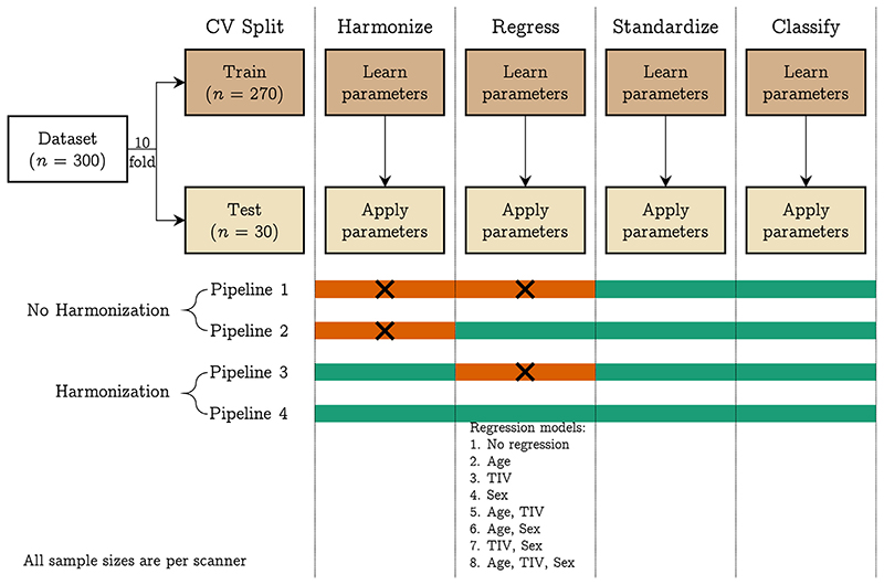
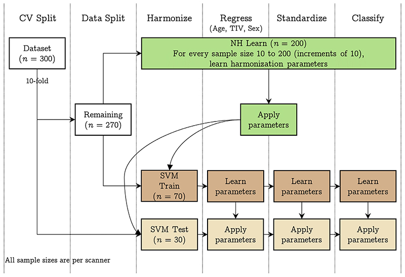
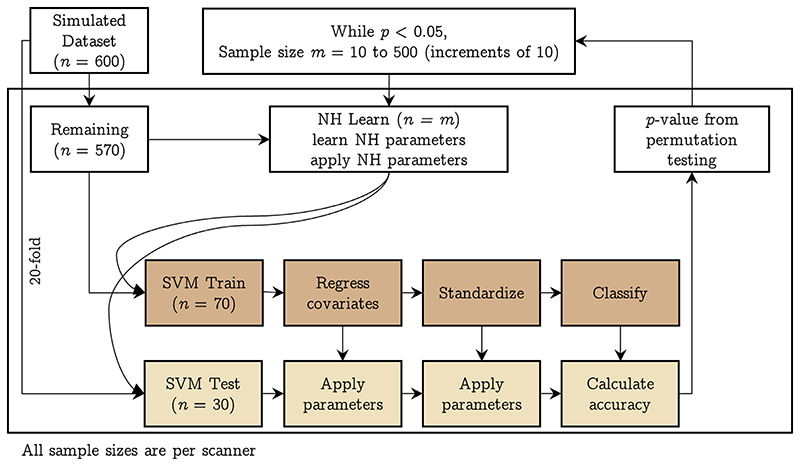
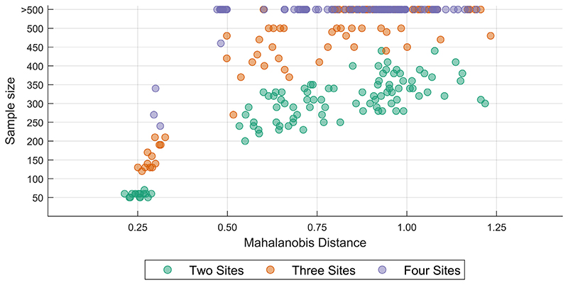
When data is pooled across multiple sites, the extracted features are confounded by site effects. Harmonization methods attempt to correct these site effects while preserving the biological variability within the features. However, little is known about the sample size requirement for effectively learning the harmonization parameters and their relationship with the increasing number of sites. In this study, we performed experiments to find the minimum sample size required to achieve multisite harmonization (using neuroHarmonize) using volumetric and surface features by leveraging the concept of learning curves. Our first two experiments show that site-effects are effectively removed in a univariate and multivariate manner; however, it is essential to regress the effect of covariates from the harmonized data additionally. Our following two experiments with actual and simulated data showed that the minimum sample size required for achieving harmonization grows with the increasing average Mahalanobis distances between the sites and their reference distribution. We conclude by positing a general framework to understand the site effects using the Mahalanobis distance. Further, we provide insights on the various factors in a cross-validation design to achieve optimal inter-site harmonization.

Keywords: Cross-validation; Harmonization; Mahalanobis distance; Multisite; Neuroimaging; Sample size.

Fig. 1

Pipelines implemented in experiment 2: we trained a linear SVM classifier to predict the scanner from raw and harmonized structural features; additionally, we explored eight different regression models where we regressed the effect of different confounding variables from the structural features; the four pipelines have four different modules: harmonization, regression, standardization, and classification; the steps indicated with orange color were not performed in that pipeline. The 10-fold cross-validation was repeated 50 times and an additional 50 repeats of permutation testing (i.e., 100 repeats of permutation) were performed to assess whether the classification performance was above chance level. [color version of this figure is available online]. (For interpretation of the references to colour in this figure legend, the reader is referred to the web version of this article.)

Fig. 2

Pipeline implemented in experiment 3: we trained a linear SVM classifier to predict the scanner after using different samples sizes to achieve harmonization of structural features; first, we performed a 10-fold split on the data resulting in 30 samples per scanner (SVM Test) and 270 samples per scanner. The 270 samples were next split into 200 samples per scanner (NH learn) and 70 samples per scanner (SVM Train). For every sample size 10 to 200, at increments of 10, we learnt the harmonization parameters using NH learn and applied it to SVM Train and SVM Test samples. Then, after regressing the effect of age, TIV, and sex, we standardized the SVM Train data (and applied the regression and standardization parameters to SVM Test) and trained a linear SVM classifier to predict the scanner. Model performance was assessed on SVM Test dataset. The 10-fold cross-validation was repeated 50 times and an additional 50 repeats of permutation testing (i.e., 100 repeats of permutation) were performed to assess whether the classification performance was above chance level. [color version of this figure is available online]. (For interpretation of the references to colour in this figure legend, the reader is referred to the web version of this article.)

Fig. 3

Pipeline implemented in experiment 4: using simulated data, we trained a linear SVM classifier to predict the scanner after using different samples sizes to achieve harmonization of structural features; we performed a 20-fold split on the data resulting in 30 samples per scanner (SVM Test) and 570 remaining samples per scanner. The 570 samples were next split into 500 samples per scanner (NH learn) and 70 samples per scanner (SVM Train). For every sample size 10 to 500, at increments of 10, we learnt the harmonization parameters using NH learn and applied it to SVM Train and SVM Test samples. Then, after regressing the effect of age, TIV, and sex, we standardized the SVM Train data (and applied the regression and standardization parameters to SVM Test) and trained a linear SVM classifier to predict the scanner. Model performance was assessed on SVM Test dataset. The 20-fold cross-validation was repeated 50 times and an additional 50 repeats of permutation testing (i.e., 100 repeats of permutation) were performed to assess whether the classification performance was above chance level. The whole process was repeated for every sample size in NH learn till the classification performance was above chance level. [color version of this figure is available online]. (For interpretation of the references to colour in this figure legend, the reader is referred to the web version of this article.)

Fig. 4

Summary of p-values from two sample Kolmogorov-Smirnov (KS) test between pairs of scanners for gray matter volumes from the left hemisphere. Each sub-plot indicates the p-values before (lower triangle) and after harmonization (upper triangle) between all pairs of scanners; the diagonal elements are shaded in a constant color to help distinguish lower and upper triangles. Each cell is color coded based on their p-value and only values smaller than 0.05 are shown. See Table S1 for the full names of the ROIs. Note that AOMIC dataset has been abbreviated to “AOM”, BNUBeijing dataset has been abbreviated to “BNUB”, and “NIMHANS” dataset has been abbreviated to “NIM”. [color version of this figure is available online].

Fig. 5

Summary of p-values from two sample Kolmogorov-Smirnov (KS) test between pairs of scanners for gray matter volumes from the right hemisphere. Each sub-plot indicates the p-values before (lower triangle) and after harmonization (upper triangle) between all pairs of scanners; the diagonal elements are shaded in a constant color to help distinguish lower and upper triangles. Each cell is color coded based on their p-value and only values smaller than 0.05 are shown. See Table S1 for the full names of the ROIs. Note that AOMIC dataset has been abbreviated to “AOM”, BNUBeijing dataset has been abbreviated to “BNUB”, and “NIMHANS” dataset has been abbreviated to “NIM”. [color version of this figure is available online].

Fig. 6

Summary of experiment 2 for representative cases for a) two sites, b) three sites, c) four sites, and d) five sites taken at a time; The x-axis indicates the model type − raw (R) data and harmonized (H) data with different combinations of covariates being regressed while the y-axis indicates the 10-fold cross-validated percentage accuracy of SVM classifier; the training and test accuracy points are across 50 repeats of 10-fold cross-validation while the permutation accuracy points are across 100 repeats of 10-fold cross-validation; the asterisk mark indicates models where the permutation testing p-value was less than 0.05; the theoretical chance level accuracy is indicated with a dashed black line [color version of this figure is available online].

Fig. 7

Average Mahalanobis distances between combinations of sites before and after regression of age, TIV, and sex for raw data; for any site combination, we first created a reference distribution using the overall mean and the pooled covariance; then, we calculated the distances of each site from this reference distribution and summarized it as the overall average; the x-axes indicate the different feature categories − gray matter volumes, cortical thickness (CT), fractal dimension (FD), sulcal depth (SD), and gyrification index (GI). Note that the AOMIC dataset has been abbreviated to “AOM,” BNUBeijing dataset has been abbreviated to “BNUB”, and the NIMHANS dataset has been abbreviated to “NIM”. [color version of this figure is available online].

Fig. 8

Summary of learning curves for volumetric features for two-site combinations; the orange points indicate the test accuracy of the SVM classifier (50 repeats of 10-fold cross-validation), the purple points indicate the permutation test accuracy of the SVM classifier (100 repeats of 10-fold cross-validation), while the dashed black line indicates the theoretical chance accuracy level; the x-axis indicates the sample size used for learning harmonization parameters (“NHLearn”) while the y-axis indicates the test accuracy in percentage. The title of each figure indicates the site-combinations, the average Mahalanobis distance (MD) of the two sites from the reference, and the sample size required for learning harmonization parameter (n) such that the SVM classifier performance was no different than chance level; the accuracies that were above chance are marked with an orange asterisk mark [color version of this figure is available online]. (For interpretation of the references to colour in this figure legend, the reader is referred to the web version of this article.)

Fig. 9

Plot of the sample size required for achieving inter-site harmonization for a range of Mahalanobis distances for two-, three-, and four-site scenarios; the features were simulated using means and covariances from fractal dimension features from real data (see text for details) [color version of this figure is available online]. (For interpretation of the references to colour in this figure legend, the reader is referred to the web version of this article.)

References

1. Ardekani BA. A New Approach to Symmetric Registration of Longitudinal Structural MRI of the Human Brain. bioRxiv. 2018 doi: 10.1101/306811. - DOI - PMC - PubMed
1. Ardekani BA, Bachman AH. Model-based automatic detection of the anterior and posterior commissures on MRI scans. Neuroimage. 2009;46:677–682. doi: 10.1016/j.neuroimage.2009.02.030. - DOI - PMC - PubMed
1. Ardekani BA, Kershaw J, Braun M, Kanuo I. Automatic detection of the mid-sagittal plane in 3-D brain images. IEEE Trans Med Imaging. 1997;16:947–952. doi: 10.1109/42.650892. - DOI - PubMed
1. Beer JC, Tustison NJ, Cook PA, Davatzikos C, Sheline YI, Shinohara RT, Linn KA. Longitudinal ComBat: a method for harmonizing longitudinal multi-scanner imaging data. Neuroimage. 2020;220:117129. doi: 10.1016/j.neuroimage.2020.117129. - DOI - PMC - PubMed
1. Biswal BB, Mennes M, Zuo X-N, Gohel S, Kelly C, Smith SM, Beckmann CF, Adelstein JS, Buckner RL, Colcombe S, Dogonowski A-M, et al. Toward discovery science of human brain function. PNAS. 2010;107:4734–4739. doi: 10.1073/pnas.0911855107. - DOI - PMC - PubMed
Publication types