Review
. 2023 Jan;27(1):43-64.
doi: 10.1016/j.tics.2022.10.004. Epub 2022 Nov 24.

Contextual inference in learning and memory

Affiliations
Review

Contextual inference in learning and memory

James B Heald et al. Trends Cogn Sci. 2023 Jan.

Abstract

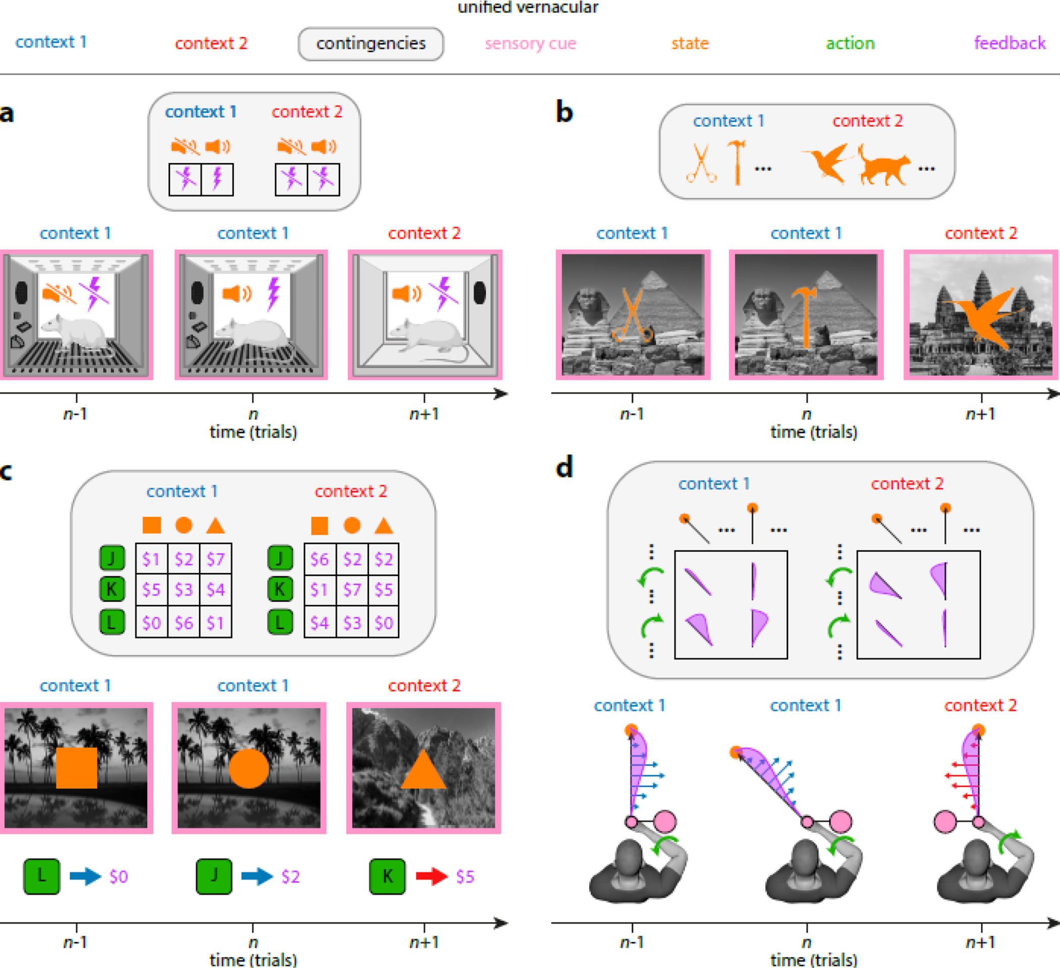
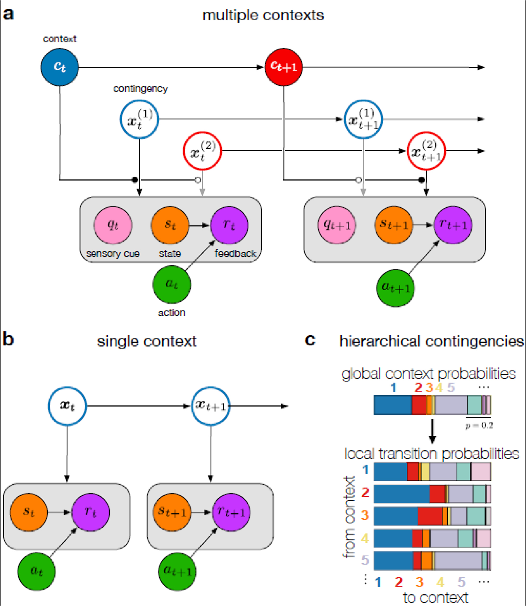
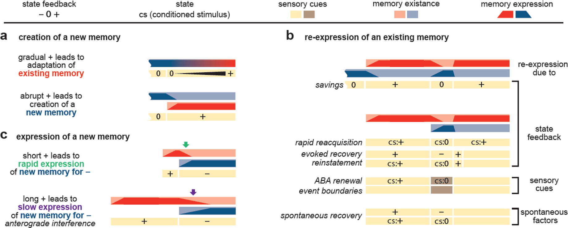
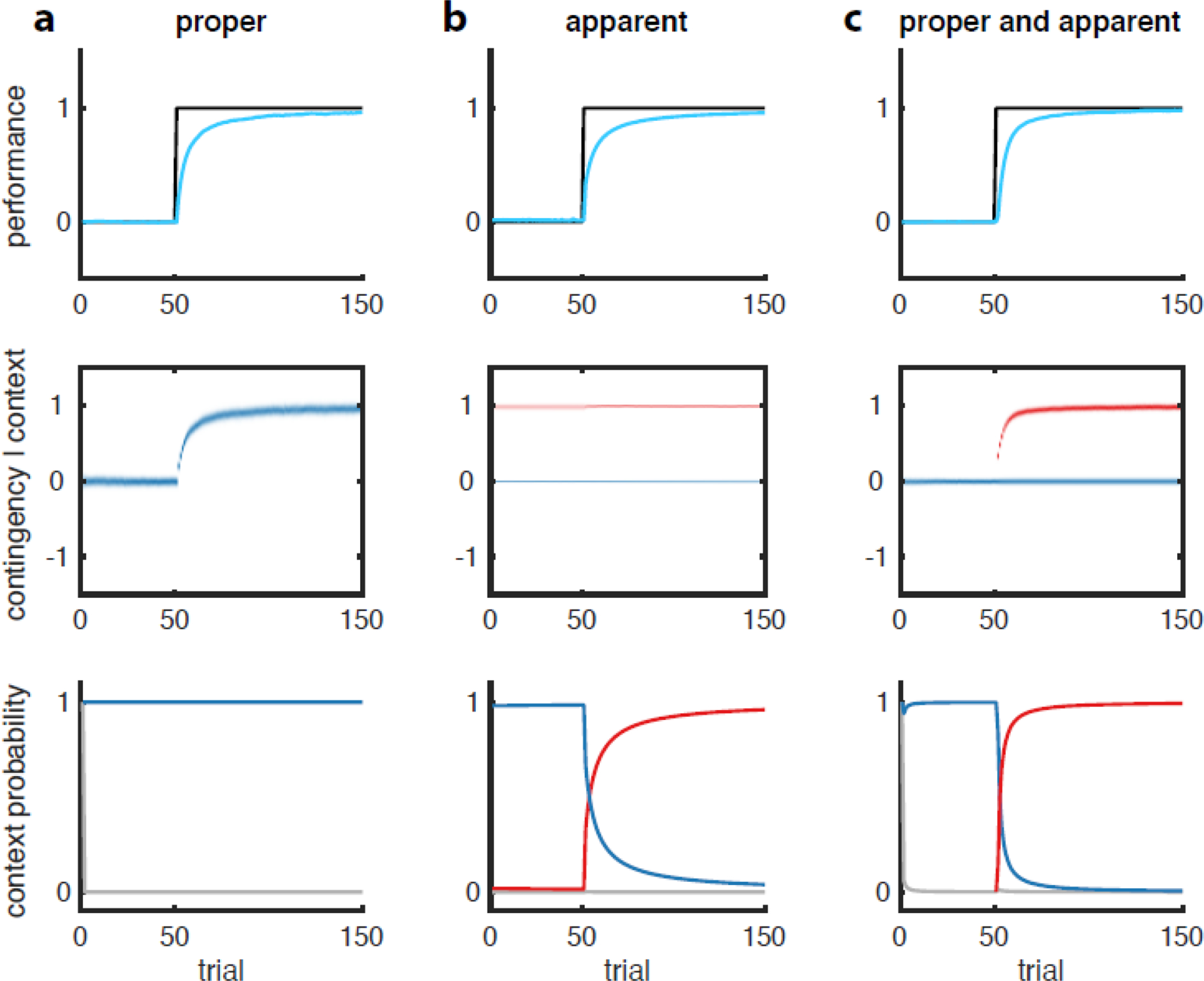
Context is widely regarded as a major determinant of learning and memory across numerous domains, including classical and instrumental conditioning, episodic memory, economic decision-making, and motor learning. However, studies across these domains remain disconnected due to the lack of a unifying framework formalizing the concept of context and its role in learning. Here, we develop a unified vernacular allowing direct comparisons between different domains of contextual learning. This leads to a Bayesian model positing that context is unobserved and needs to be inferred. Contextual inference then controls the creation, expression, and updating of memories. This theoretical approach reveals two distinct components that underlie adaptation, proper and apparent learning, respectively referring to the creation and updating of memories versus time-varying adjustments in their expression. We review a number of extensions of the basic Bayesian model that allow it to account for increasingly complex forms of contextual learning.

Keywords: Bayesian inference; context-dependent learning; learning; memory.


Conflict of interest statement

Declaration of interests D.M.W. is a consultant to CTRL-Labs Inc., in the Reality Labs Division of Meta. This entity did not support or influence this work. The authors declare no other competing interests.

Figures

Fig. 1 |
Fig. 1 |. Elements of contextual learning in different domains.
Top row shows key elements of contextual learning (color coded; see also Box 1), panels show how they apply to specific domains. Three consecutive trials in a typical classical conditioning (a), episodic memory (b), instrumental learning (c) and motor adaptation (d) task. For each task, the first two trials (trials n−1 and n) are in context 1 (blue), and the last trial (trial n+1) is in context 2 (red). Each context can be associated with an observed sensory cue (pink, conditioning chamber in a, background image in b and c, and orientation of virtual tool in d). The sensory cue is informative of the context but is not directly related to task performance. On each trial, the participant observes a state (orange, presence or absence of auditory tone in a, foreground image in b and c, and target location in d). The participant selects an action (green, no action is taken in a and b, discrete button press in c, and continuous elbow joint torque in d). Given the state and action (if applicable), the participant receives feedback (purple, presence or absence of foot shock in a, no feedback in b, monetary reward in c, and observed hand trajectory in d). The relationship between state, action and feedback is determined by the context-specific contingencies (gray box). The straight arrows in d show velocity-dependent forces produced by the handle of the robot (not shown) grasped by the participant. Note that some of the specific experimental paradigms only use a subset of these ingredients. For example, actions are usually not considered in classical conditioning (a) or (the study phase of) episodic memory experiments (b; in this case, typically there is not even feedback, but see [142]), motor learning experiments (d) often have only one state (i.e. the same target across all trials) for each context, and many paradigms do not use any context-specific sensory cues. In addition, historically, the same term has come to refer to different concepts in different domains: for example, the term “state” as used in state-space models of motor learning [72, 114, 128] refers to the concept that we here call “contingency”, while we reserve the use of the term “state” in a sense that is closest to that used in reinforcement learning [120]. Finally, sometimes terms other than “context” are used to express the same concept (e.g. “task set” or “abstract rule” in economic decision making).
Fig. 2 |
Fig. 2 |. Internal model of the environment commonly imputed to learners.
a-b. Graphical models underlying multiple context (a) and single context models (b). Temporal changes in variables (circles) are formalized by introducing multiple nodes for them, each corresponding to the value of the variable in a different time step (subscript), and then introducing directed edges (horizontal arrows) between them to describe how their future values depend on their past values (i.e. internal dynamics). The value of a variable in a given time step can also depend on other variables in the same time step (vertical arrows). a. Multiple-context model [12, 13, 58, 59, 95]. Contexts (top nodes, color represents the identity of the active context) evolve according to Markovian transition probabilities. Each context has its own contingency (only two shown for simplicity; in general, the number of contexts and contingencies can be unbounded). Contexts can also be associated with sensory cues (pink) of which the appearance probabilities are also dictated by the context-specific contingencies. Only the contingency associated with the active context influences the observed sensory cue, state (orange) and feedback (purple) variables (gating by context, black vs. gray arrows). Feedback can depend on both an observed state and an action (green). In general, the active contingency can also affect the next context transition (for clarity, arrows not shown). In addition, states may not be directly observable and may have their own (action-dependent) dynamics [120] (also not shown for clarity). Gray box indicates that the contingency, xt, determines the joint distribution of the variables inside the box (here: qt, st and rt) b. Single-context model [57, 119, 116] in which only a single contingency exists. c. Hierarchical contingencies: an example of transition probabilities (as generated by a hierarchical Dirichlet process). The set of probabilities for transitioning ‘from’ each context (bottom, horizontal multicolored bars, with the width of each stripe showing the probability of transitioning to each ‘to’ context) is a variation on a global set of probabilities (top). This way, learning about the local transition probabilities in a particular context informs inferences about global transition probabilities, in turn informing inferences about other local transition probabilities, even for context transitions that have not yet been observed.
Fig. 3 |
Fig. 3 |. Classical paradigms explained by contextual inference.
Each paradigm is schematically represented by three rows (two rows in panel a, top). The bottom row (rows in panel b) with yellow/brown colored bars shows the time course of the experiment in terms of state feedback (positive, +, negative, −, null, 0, or absent, blank), sensory cues (yellow and brown), and state (CS). For motor control, +, 0, and − reflect the strength and direction of a perturbation applied to the hand during reaching. For conditioning +, and 0 reflect the presence/absence of a US. The top two rows (top row in panel a, top) with red/blue colored bars show the memories that are relevant to the experiment (red for +, blue for 0 or −); for each memory, the bar with pale background extends from the time the memory was created until the end of the experiment (scalloped edge reflects a pre-existing memory). Dark shading within each bar shows the expression of the corresponding memory at each point in time (the height of the dark shading represents the level of expression, between 0 and 1, with the expression across existing contexts summing to 1). Below we highlight the paradigms (see main text and Box 3 for details of the paradigms and explanation of the mechanisms). a. Top: for a gradually introduced perturbation (black expanding triangle in second row) the existing memory is updated (blue changing to red in first row). Bottom: memory creation occurs for an abruptly introduced perturbation. b. Paradigms in which an initially learned memory (red) is re-expressed later in the paradigm after another memory has been expressed. Re-expression can rely on the state feedback, sensory cue or spontaneous factors. c. New memory expression. Anterograde interference, in which learning a second contingency (here, − perturbation) is slower if another contingency (here, + perturbation) has initially been learned, with the amount of interference increasing with the length of initial learning (long + vs. short +), that is when the environment is less volatile. Green and purple arrows to point to rapidly vs. slowly changing levels of memory expression, respectively.
Fig. 4 |
Fig. 4 |. Identical learning curves can arise due to proper or apparent learning, or their combination.
Simulations of a model of contextual learning [13] in response to a step change in a (deterministic) contingency (black line, top row) under three different scenarios (a-c). The three scenarios unfold under different parameter settings and initial conditions (e.g. 1 vs. 2 memories). Task performance (top row, cyan) is a mixture of the inferred contingency distributions for each context (middle row, blue and red). For simplicity, each inferred contingency directly determines a response magnitude appropriate for the corresponding context. The mixture is weighted by the associated context probabilities (bottom row, blue and red – gray shows the probability a potential novel context). a. Pure proper learning: the “contingency” corresponding to the relevant state (e.g. defined by the presentation of the CS, or a movement target) is simply a scalar, such as the probability of receiving the US as feedback in that state, or the magnitude of force perturbation when reaching to that target. In naive subjects, the estimate of this contingency is initially 0, and over training it is increased as the CS is consistently paired with US, or the force perturbation with the target (middle row). This gives rise to a classical learning curve. Note that in this example, contextual inference plays no role whatsoever, as (the simulated subject assumes) there is only a single context at play at all times of which the probability can thus only be constant one at all times (bottom row). b. Pure apparent learning: an existing (red) memory whose contingency has previously been updated to some non-zero level (here taken to be 1, for simplicity) is expressed more over time, relative to a baseline memory (blue, taken to be at zero), as its associated context is inferred to be active with increasing probability (bottom row, probability of red context increases). Thus, memory updating plays no role here, as the estimated contingencies for both contexts are constant through time (middle row). c. Mixture of proper and apparent learning: a new (red) memory is created and updated but also expressed more over time. Critically, these distinct forms of learning can produce identical adaptation curves (a-c, top panels), despite having radically different internal representations (middle and bottom panels).

References

    1. Courville AC, Daw ND, and Touretzky DS (2006). Bayesian theories of conditioning in a changing world. Trends in Cognitive Sciences 10, 294–300. - PubMed
    1. Redish AD, Jensen S, Johnson A, and Kurth-Nelson Z (2007). Reconciling reinforcement learning models with behavioral extinction and renewal: implications for addiction, relapse, and problem gambling. Psychological Review 114, 784–805. - PubMed
    1. Gershman SJ, Blei DM, and Niv Y (2010). Context, learning, and extinction. Psychological Review 117, 197–209. - PubMed
    1. Howard MW and Kahana MJ (2002). A distributed representation of temporal context. Journal of Mathematical Psychology 46, 269–299.
    1. Zacks JM, Speer NK, Swallow KM, Braver TS, and Reynolds JR (2007). Event perception: a mind-brain perspective. Psychological Bulletin 133, 273–293. - PMC - PubMed

Publication types