Standardized multi-omics of Earth's microbiomes reveals microbial and metabolite diversity

Abstract

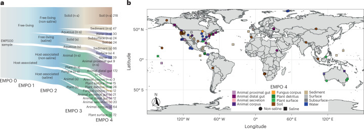
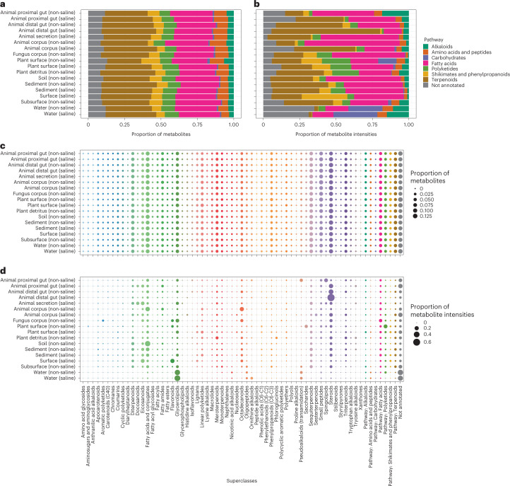
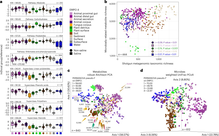
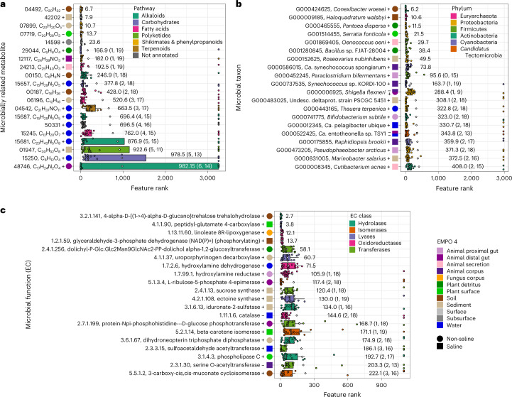
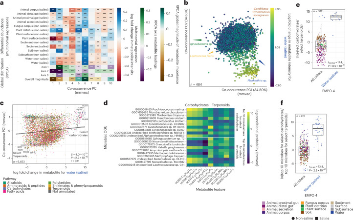
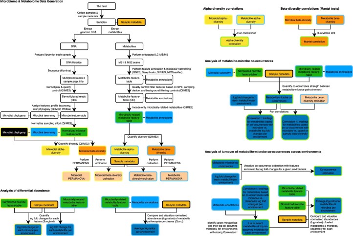
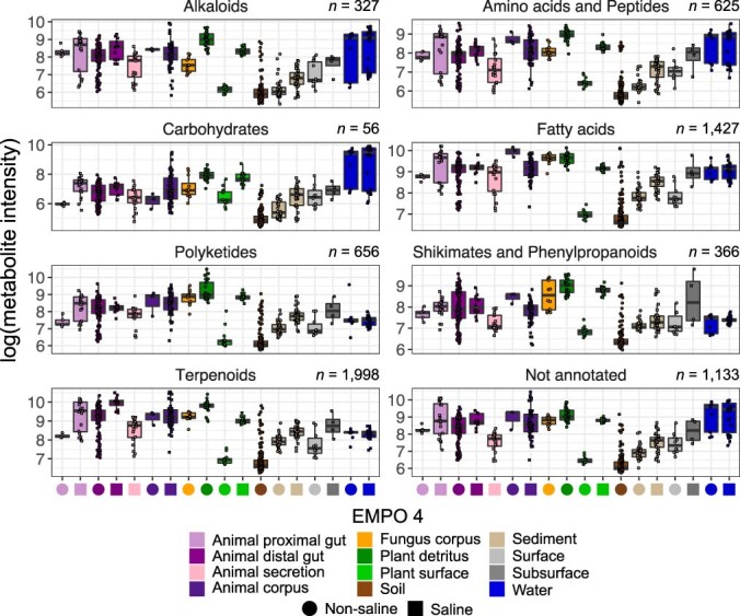
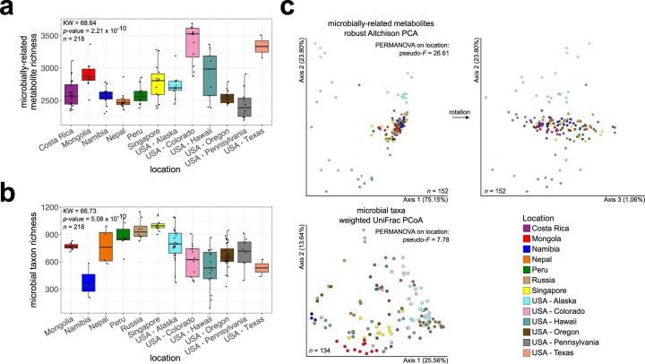
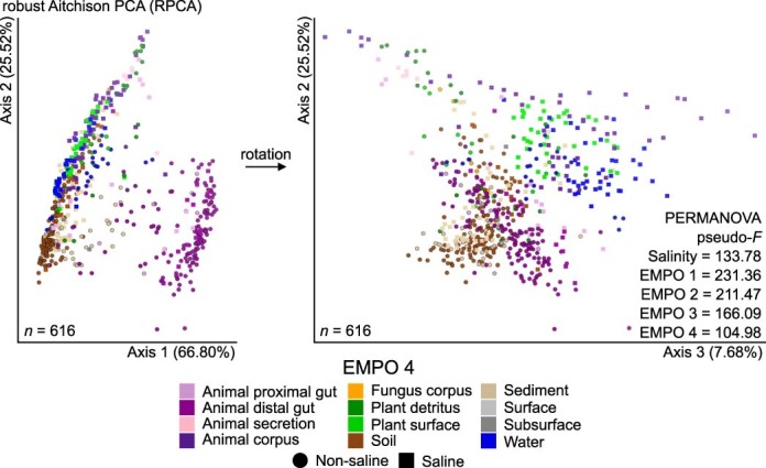
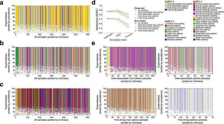
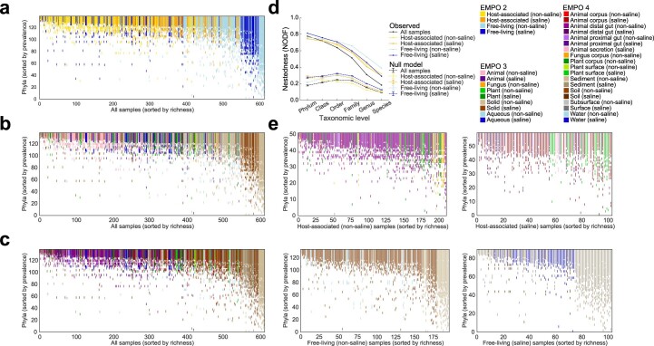
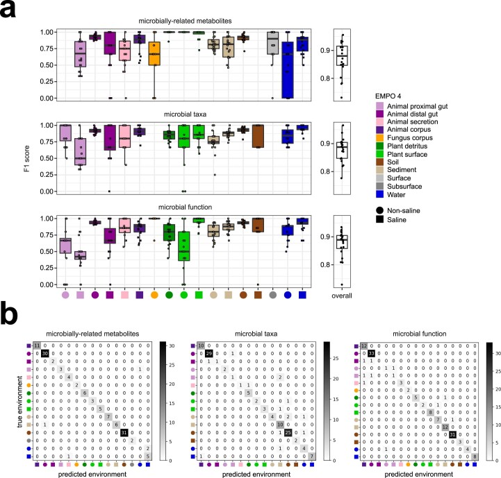
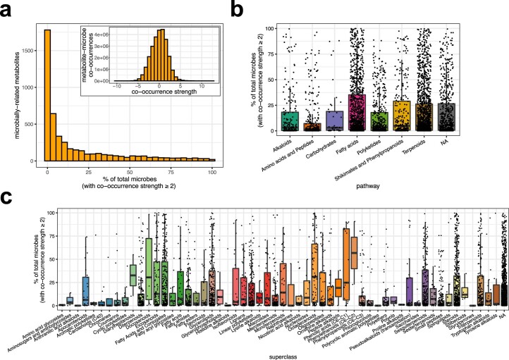
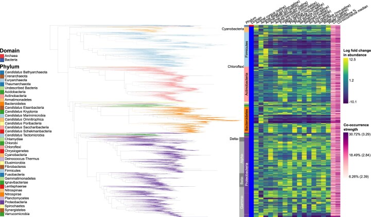
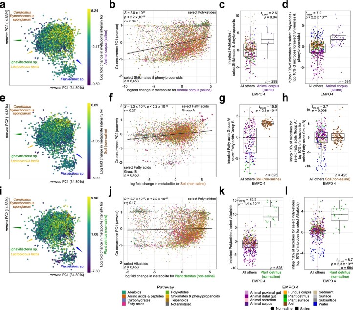
Despite advances in sequencing, lack of standardization makes comparisons across studies challenging and hampers insights into the structure and function of microbial communities across multiple habitats on a planetary scale. Here we present a multi-omics analysis of a diverse set of 880 microbial community samples collected for the Earth Microbiome Project. We include amplicon (16S, 18S, ITS) and shotgun metagenomic sequence data, and untargeted metabolomics data (liquid chromatography-tandem mass spectrometry and gas chromatography mass spectrometry). We used standardized protocols and analytical methods to characterize microbial communities, focusing on relationships and co-occurrences of microbially related metabolites and microbial taxa across environments, thus allowing us to explore diversity at extraordinary scale. In addition to a reference database for metagenomic and metabolomic data, we provide a framework for incorporating additional studies, enabling the expansion of existing knowledge in the form of an evolving community resource. We demonstrate the utility of this database by testing the hypothesis that every microbe and metabolite is everywhere but the environment selects. Our results show that metabolite diversity exhibits turnover and nestedness related to both microbial communities and the environment, whereas the relative abundances of microbially related metabolites vary and co-occur with specific microbial consortia in a habitat-specific manner. We additionally show the power of certain chemistry, in particular terpenoids, in distinguishing Earth's environments (for example, terrestrial plant surfaces and soils, freshwater and marine animal stool), as well as that of certain microbes including Conexibacter woesei (terrestrial soils), Haloquadratum walsbyi (marine deposits) and Pantoea dispersa (terrestrial plant detritus). This Resource provides insight into the taxa and metabolites within microbial communities from diverse habitats across Earth, informing both microbial and chemical ecology, and provides a foundation and methods for multi-omics microbiome studies of hosts and the environment.

Fig. 1. Environment type and provenance of samples.

a, Distribution of samples (n = 880) among the Earth Microbiome Project Ontology (EMPO version 2) categories. EMPO recognizes strong axes of variation in microbial communities, and thus organizes all microbial environments (level 4) on the basis of host association (level 1), salinity (level 2), host taxon (for host-associated) or phase (free-living) (level 3). For EMPO 3 and EMPO 4: n-s, non-saline; s, saline. Colours indicate environments. Numbers indicate sample counts for each environment. Made with JSFiddle. b, Geographic distribution of samples with points coloured by EMPO 4. Points are transparent to highlight cases where multiple samples derive from a single location. We note here that our intent was to sample across environments rather than geography, in part because we previously showed that microbial community composition is more influenced by the former rather than the latter, but also to motivate finer-grained geographic exploration as sample analyses decrease in cost. Extensive information about each sample set is described in Supplementary Table 1. Made with Natural Earth.

Fig. 2. Distribution of microbially related secondary metabolite pathways and superclasses among environments.

a–d, Individual metabolites are represented by their higher-level classifications. Both chemical pathway and chemical superclass annotations are shown on the basis of presence/absence (a,c) and relative intensities (b,d) of molecular features, respectively. For superclass annotations in c and d, we included pathway annotations (when possible) for metabolites where superclass annotations were not available, and colours identify superclasses and pathways.

Fig. 3. Structural-level associations between microbially related secondary metabolites and specific environments.

a, Differential abundance of metabolites across environments. For each panel, the y axis represents the natural log-ratio of the intensities of ingroup metabolites divided by the intensities of reference group metabolites (that is, pathway reference: Amino acids and peptides, n = 615; superclass reference: Flavonoids, n = 42). The number of metabolites in each ingroup and the chi-squared statistic from a Kruskal–Wallis (KW) test for differences across environments are shown. For each test, n = 606 samples and P < 2.2 × 10⁻¹⁶. Boxplots are Tukey’s, where the centre indicates the median, lower and upper hinges the first and third quartiles, respectively, and each whisker is 1.5× the interquartile range (IQR) from its hinge. b, Relationship between metabolite richness and microbial taxon richness, with significant correlations noted. P values are from two-tailed tests and were adjusted using the Benjamini-Hochberg procedure. c, Turnover in composition of metabolites across environments, visualized using RPCA, showing samples separated on the basis of metabolite abundances. Shapes represent samples. Arrows represent metabolites and are coloured by chemical pathway. The direction and magnitude of each arrow corresponds to the correlation between the metabolite’s abundance and the ordination axes. Samples close to arrow heads have strong positive associations, samples at arrow origins have no association, and those beyond arrow origins have strong negative associations. Metabolites are described in Supplementary Table 4. Metabolites annotated in red and purple were also highly differentially abundant across environments (Supplementary Table 3), and those in purple were also identified as important in co-occurrence analyses (Fig. 4). d, Turnover in composition of microbial taxa across environments, visualized using PCoA of weighted UniFrac distances. For c and d, results from PERMANOVA (999 permutations) for each level of EMPO are shown (all tests had P = 0.001; group sizes for metabolites: k_EMPO1 = 2, k_EMPO2 = 4, k_EMPO3 = 9, k_EMPO4 = 18; group sizes for microbial taxa: k_EMPO1 = 2, k_EMPO2 = 4, k_EMPO3 = 9, k_EMPO4 = 19). Sample sizes in a refer to metabolites, but in all other panels refer to samples.

Fig. 4. Machine-learning analysis of microbially related metabolites, microbial taxa and microbial functions, highlighting the top 20 most impactful features for each dataset.

a, The top 20 most impactful microbially related metabolites. Features are coloured by metabolite pathway. Metabolites in bold font are those also identified as important in differential abundance analysis (Supplementary Table 3). b, The top 20 most impactful microbial taxa (that is, OGUs). Taxa are coloured by phylum. c, The top 20 most impactful microbial functions (that is, KEGG ECs). Boxplots are in the style of Tukey, where the centre line indicates the median, lower and upper hinges the first and third quartiles, respectively, and each whisker is 1.5× IQR from its respective hinge. Enzymes are coloured by class. For all features, ranks are based on impacts derived from SHAP values. Associations with environments are indicated, where + indicates a positive association and – indicates a negative association based on feature abundances. Diamonds and values to the right of boxes indicate means. Values in parentheses indicate (1) the number of iterations (n = 20) in which a feature had no impact and (2) the number of iterations in which the reported association was observed, for cases in which values were <20. Environments are described by the Earth Microbiome Project Ontology (EMPO 4).

Fig. 5. Metabolite–microbe co-occurrences vary across environments.

a, Correlation between metabolite loadings from the co-occurrence ordination (that is, co-occurrence PCs) and (1) log fold changes in metabolite abundances across environments, (2) metabolite loadings from the ordination in Fig. 3d (that is, Global distribution, axes 1–3) and (3) a vector representing the overall magnitude of microbial taxon abundances from the ordination in Fig. 3d (that is, Global distribution, Overall magnitude). Values are Spearman correlation coefficients. Asterisks indicate significant correlations (*P < 0.05, **P < 0.01, ***P < 0.001). b, The relationship between log fold changes in metabolite abundance with respect to ‘Water (non-saline)’ and the first three PCs of the co-occurrence ordination. Points represent metabolites, and the distance between metabolites indicates similarity in their co-occurrences with microbial taxa. Metabolites are coloured on the basis of log fold changes with respect to ‘Water (non-saline)’. Arrows represent specific microbial taxa (colours), distances between arrow tips indicate similarity in their co-occurrence with specific metabolites, and the direction of each arrow indicates which metabolites each microbe co-occurs most strongly with. c, The relationship between log fold changes in metabolite abundances with respect to ‘Water (non-saline)’ and loadings for metabolites on PC1 of the co-occurrence ordination. The correlation is one example from a. Metabolites are coloured by pathway. Select carbohydrates (excluding glycosides) (the focal group) and select terpenoids (the reference group) are highlighted. d, The top 10 co-occurring microbial taxa for all select carbohydrates and all select terpenoids, with a heat map showing co-occurrence strength. e, Log-ratio of metabolite intensities for select carbohydrates and select terpenoids. f, Log-ratio of abundances of the top 10 microbial taxa associated with select carbohydrates and with select terpenoids. For e and f, points represent samples, and results from a t-test comparing ‘Water (saline)’ vs all other environments are shown. Boxplots are Tukey’s, where the centre indicates the median, lower and upper hinges the first and third quartiles, respectively, and each whisker represents 1.5× IQR from its hinge. For a, c, e and f, P values are from two-sided tests. For a and c, P values were adjusted using the Benjamini-Hochberg procedure.

Extended Data Fig. 1. Diagrammatic overview of multi-omics analyses performed using the EMP500 dataset.

The process begins with data generation for both the microbiome and metabolome, which is then followed by analysis of differential abundance of both microbial taxa and microbially-related metabolites across environments. To begin multi-omics integration, correlations between alpha- and beta-diversity are explored, followed by explicit co-occurrence analysis of metabolite-microbe pairs. The results from analysis of co-occurrence are then combined with those from analysis of differential abundance, to reveal strong patterns of metabolite-microbe turnover across environments. Throughout the diagram, artifacts derived from microbial data are outlined in yellow, those derived from metabolite data are outlined in blue, and those derived from co-occurrence analysis are outlined in green.

Extended Data Fig. 2. Relative abundance of microbially-related metabolite pathways, highlighting among-sample variation for each environment.

These data are shown as a complement to those in Fig. 2b of the main text. We note that as abundance data were not normalized (for example, by using log-ratios as in Fig. 3a), caution should be used in interpreting differences among environments. Boxplots are in the style of Tukey, where the center line indicates the median, lower and upper hinges the first- and third quartiles, respectively, and each whisker 1.5 x the interquartile range (IQR) from its respective hinge. For each panel, n = 618 biologically independent samples, and the number of metabolites per pathway is shown.

Extended Data Fig. 3. Microbially-related metabolite and microbial taxon composition among geographic locations for all non-saline soil samples.

a, Metabolite richness. b, Microbe richness. For a and b, the chi-squared statistic from a Kruskal-Wallis rank sum test for differences in richness across environments is shown (that is, each test had p-value < 2.2 x 10^-16). c, Beta-diversity based on metabolites (upper panel) and microbes (lower panel). Results from PERMANOVA tests (n = 999 permutations) for variance explained by salinity as well as each level of EMPO are shown; p-value = 0.001 for all tests.

Extended Data Fig. 4. Clustering of samples by environments highlighting beta-diversity based on shotgun metagenomics data for microbial functions.

Robust Aitchison PCA with samples colored by EMPO 4 and shaped by salinity. Features are KEGG ECs (that is, enzymes). Results from PERMANOVA tests (n = 999 permutations) for variance explained by salinity as well as each level of EMPO are shown; p-value = 0.001 for all tests.

Extended Data Fig. 5. Nestedness of community composition based on microbially-related metabolites.

a, Presence-absence of superclasses across samples, with superclasses (rows) sorted by prevalence and samples (columns, n = 618) sorted by richness. With increasing sample richness, superclasses tended to be gained but not lost (SES = 108.61, p-value < 0.0001 vs. a null model from a two-tailed test; nestedness measure based on overlap and decreasing fills [NODF] statistic = 0.87). Samples are colored by EMPO 2. b, As in a but with samples colored by EMPO 3. c, As in a but with samples colored by EMPO 4. d, Nestedness as a function of annotation level, from superclass to molecular formula, across all samples and within environments based on EMPO 2. Also shown are median null model NODF scores (± s.d.) for all samples, as well as samples at each level of EMPO 2. NODF measures the average fraction of metabolites from less diverse communities that occur in more diverse communities. All environments at all annotation levels examined were more nested than expected randomly, with nestedness higher at higher annotation levels (p-value < 0.0001 for all comparisons, from two-tailed tests). e, As in c but with each environment at EMPO 2 shown separately, with samples colored by EMPO 4.

Extended Data Fig. 6. Nestedness of community composition based on microbial taxa.

Presence-absence of phyla across samples, with phyla (rows) sorted by prevalence and samples (columns, n = 612) sorted by richness. With increasing sample richness, phyla tended to be gained but not lost (SES = 91.86, p-value < 0.0001 vs. a null model; nestedness measure based on overlap and decreasing fills [NODF] statistic = 0.78). Samples are colored by EMPO 2. b, As in a but with samples colored by EMPO 3. c, As in a but with samples colored by EMPO 4. d, Nestedness as a function of taxonomic level, from phylum to species, across all samples and within environments based on EMPO 2. Also shown are median null model NODF scores (± s.d.) for all samples, as well as samples at each level of EMPO 2. NODF measures the average fraction of taxa from less diverse communities that occur in more diverse communities. All environments at all taxonomic levels examined were more nested than expected randomly, with nestedness higher at higher taxonomic levels (p-value < 0.0001 for all comparisons, from two-tailed tests). e, As in c but with each environment at EMPO 2 shown separately, with samples colored by EMPO 4.

Extended Data Fig. 7. Machine-learning analysis of microbially-related metabolites, microbial taxa, and microbial functions, highlighting per-environment classification performance.

a, The F1 score (that is, which considers precision and recall) for each environment as well as overall across all environments. For each data layer, every environment is represented by n = 20 iterations. b, Confusion matrices for each data layer highlighting which pairs of environments are confused. Boxplots are in the style of Tukey, where the center line indicates the median, lower and upper hinges the first- and third quartiles, respectively, and each whisker 1.5 x the interquartile range (IQR) from its respective hinge. For all analyses, environments are described by the Earth Microbiome Project Ontology (EMPO 4).

Extended Data Fig. 8. Summary of co-occurrence ranks for microbially-related metabolites.

a, Distribution of the percentage of microbial taxa for which co-occurrences were strong. Strong co-occurrence was defined as having a co-occurrence strength (that is, rank, or log conditional probability) ≥ 2. The overall distribution of co-occurrence strengths is shown in the inset (n = 26,784,120). For values > 0 (n = 13,851,755), the minimum = –10.17, maximum = 12.69, mean = 2.40 x 10^-18, median = 0.08, and mode = 1.22. For values ≥ 2 (n = 3,496,639), the minimum = 2.00, maximum = 12.69, mean = 2.87, median = 2.63, and mode = 4.26. b, The percentage of microbial taxa for which co-occurrences were strong (that is, ≥ 2), across metabolite pathways. c, The percentage of microbial taxa for which co-occurrences were strong (that is, ≥ 2), across metabolite superclasses. For panels b and c, points were jittered horizontally for clarity, and n = 4,765 metabolites. Boxplots are in the style of Tukey, where the center line indicates the median, lower and upper hinges the first- and third quartiles, respectively, and each whisker 1.5 x the interquartile range (IQR) from its respective hinge.

Extended Data Fig. 9. Phylogenetic relationships among microbial taxa highlighting log fold changes in abundance relative to environment, and overall co-occurrences with microbially-related metabolites.

Branches are colored by microbial phylum. Annotations include Domain and Phylum level associations (and Class for Proteobacteria), heat maps representing log fold changes in relative abundance for each environment (from songbird), and heat maps summarizing co-occurrences with microbially-related metabolites (from mmvec). Co-occurrence strength indicates (1) the percentage of all microbially-related metabolites for which the co-occurrence rank (that is, log conditional probability) was ≥ 2 (that is, strong), and (2) the median co-occurrence rank value, considering only strong values (in parentheses in the legend).

Extended Data Fig. 10. Metabolite-microbe co-occurrences reveal exhibit strong turnover across environments.

Results from three environments in addition to ‘Water (saline)’, to highlight differences driven by salinity and host-association: ‘Animal corpus (saline)’, ‘Soil (non-saline)’, and ‘Plant detritus (non-saline’). a, e, i, The relationship between log fold changes in abundance for metabolites with respect to the focal environment, and the first three co-occurrence PCs. See Fig. 5 for details. b, f, j The relationship between log fold changes in metabolite abundances with respect to the focal environment and loadings for metabolites on PC1 of the co-occurrence ordination. The correlations are examples from Fig. 5a. Metabolites are colored by pathway. Select features representing the focal group and reference group are highlighted, and are described along with the top ten co-occurring microbial taxa for each group in Supplementary Table S5. P-values are from two-tailed tests, and were adjusted for multiple comparisons using the Benjamini Hochberg procedure. c, g, k, Log-ratio of metabolite intensities for select focal group features and select reference group features with respect to the focal environment. d, h, l, Log-ratio of abundances of the top ten microbial taxa associated with focal group metabolites and with reference group metabolites, with respect to the focal environment (see Supplementary Table S5). For panels c, d, g, h, k, and l, points represent samples, and results from a two-sided t-test comparing the focal vs. all other environments are shown. Boxplots are Tukey’s, where the center indicates the median, lower and upper hinges the first- and third quartiles, respectively, and each whisker 1.5 x the interquartile range (IQR) from its hinge.

References

1. Thompson LR, et al. A communal catalogue reveals Earth’s multiscale microbial diversity. Nature. 2017;551:457–463. doi: 10.1038/nature24621. - DOI - PMC - PubMed
1. Knight R, et al. Best practices for analysing microbiomes. Nat. Rev. Microbiol. 2018;16:410–422. doi: 10.1038/s41579-018-0029-9. - DOI - PubMed
1. Proctor LM, et al. The Integrative Human Microbiome Project. Nature. 2019;569:641–648. doi: 10.1038/s41586-019-1238-8. - DOI - PMC - PubMed
1. Vangay P, et al. Microbiome metadata standards: report of the National Microbiome Data Collaborative’s workshop and follow-on activities. mSystems. 2021;6:e01194–20. - PMC - PubMed
1. Lozupone CA, Knight R. Global patterns in bacterial diversity. Proc. Natl Acad. Sci. USA. 2007;104:11436–11440. doi: 10.1073/pnas.0611525104. - DOI - PMC - PubMed
Publication types