The BrightEyes-TTM as an open-source time-tagging module for democratising single-photon microscopy

Abstract

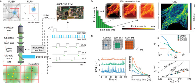
Fluorescence laser-scanning microscopy (LSM) is experiencing a revolution thanks to new single-photon (SP) array detectors, which give access to an entirely new set of single-photon information. Together with the blooming of new SP LSM techniques and the development of tailored SP array detectors, there is a growing need for (i) DAQ systems capable of handling the high-throughput and high-resolution photon information generated by these detectors, and (ii) incorporating these DAQ protocols in existing fluorescence LSMs. We developed an open-source, low-cost, multi-channel time-tagging module (TTM) based on a field-programmable gate array that can tag in parallel multiple single-photon events, with 30 ps precision, and multiple synchronisation events, with 4 ns precision. We use the TTM to demonstrate live-cell super-resolved fluorescence lifetime image scanning microscopy and fluorescence lifetime fluctuation spectroscopy. We expect that our BrightEyes-TTM will support the microscopy community in spreading SP-LSM in many life science laboratories.

Fig. 1. Concepts of FLISM and FLFS.

a In FLISM, a pulsed laser beam is focused and scanned across the sample. For each position of the laser beam, the fluorescence is collected and focused onto a SPAD array detector. Every photon produces a pulse in one of the detection channels almost instantaneously. The BrightEyes-TTM measures the arrival time of the photon with respect to the last laser pulse and the pixel, line, and frame clock of the microscope. In single-point spot-variation FLFS, the laser beam is kept steady while the photon arrival times are measured. The movement of the fluorophores results in temporal fluctuations in the intensity trace. b A super-resolution fluorescence lifetime (FLISM) image can be reconstructed from the resulting 4D dataset (x, y, t, ch). For each time bin of the TCSPC histogram, a super-resolved ISM image is reconstructed with the adaptive pixel reassignment algorithm. All the images are then recombined, and the fluorescence lifetimes are calculated for each pixel, resulting in the final FLISM image. c In spot-variation FLFS, the diffusion time as a function of the focal spot area is measured. The dimension of the focal spot can be changed by combining the photon traces coming from different detection channels. From the autocorrelations of the resulting intensity time traces, the diffusion times, and hence the diffusion modality (free diffusion, diffusion through a meshwork, or diffusion in a sample comprising isolated microdomains), can be found. Simultaneously, from the start–stop times, the fluorescence lifetime τ_fl is measured. PCR photon count rate.

Fig. 2. BrightEyes-TTM characterization and validation.

a–c Single-shot precision experiment. a Temporal schematic representation: a fixed frequency SYNC clock signal and a synchronized but delayed (in a controlled way) signal. b Unified representation of the start–stop time histograms as a function of the imposed delay between the two signals. c Single start–stop time histogram for the delay denoted by the dotted white line in the middle panel. The inset shows a magnification of the histogram for a selected temporal interval, superimposed with the Gaussian fit (red line). d, e Dual-channel single-shot precision experiment. d Temporal schematic representation: a fixed frequency SYNC clock signal and a pair of synchronized signals (channel A and channel B). The delays between all three signals are fixed. e Jitter map for each pair of channels (here, 25 channels), i.e., error in the time-difference estimation between any two channels, measured as the standard deviation of a Gaussian fit of the error distribution. The diagonal of the map represents the sigma of the single-channel single-shot precision experiment. f Normalized impulse-response functions (dark colors) and fluorescein–water solution decay histograms (light colors) for the BrightEyes-TTM and DPC-230 multi-channel card. The instrument response functions (IRFs) represent the response of the whole architecture (microscope and DAQ) to a fast (sub-nanosecond) fluorescence emission. The full-width-at-half-max values are 250 ps for the DPC-230 card and 200 ps for the BrightEyes-TTM. The decay histograms are also typically referred to as start–stop time histograms or TCSPC histograms. All single-channel measurements were done with TTM channel #12, which received the photon signal from the central element of the SPAD array detector. All start–stop histograms have 48 ps granularity (bin width).

Fig. 3. BrightEyes-TTM for FLISM.

Imaging and FLISM analysis of 100 nm fluorescent beads with a custom-built single-photon laser-scanning microscope equipped with a 5 × 5 SPAD array detector prototype. a Side-by-side comparison of confocal (left, pinhole 0.2 AU), adaptive pixel-reassignment ISM (center), and open confocal (right, pinhole 1.4 AU). AU = Airy unit. Each imaging modality shows both the intensity-based image (top-left corner) and the lifetime image (bottom-right corner). A bidimensional look-up-table represents in the lifetime images both the intensity values (i.e., photon counts) and the excited-state lifetime values (i.e., τ_fl). The intensity-based images integrate the relative 3D data (x, y, Δt) along the start–stop time dimension Δt. b Histogram distributions showing the number of pixels versus lifetime values—in violet lifetime values which fall out of the selected lifetime interval. The selected interval was chosen by visually inspecting the FLISM image. The same intervals were used for the confocal and open confocal data. The lifetime images report in violet the pixels whose lifetime is in this interval. c Zoomed regions in the white-dashed boxes, with the intensity panels re-normalized to the maximum and minimum values. d Pixel intensity phasor plots, 5% and 10% thresholds respectively in gray and color. Pixel dwell time 100 μs. Scale bars 2 μm.

Fig. 4. Fluorescence lifetime image-scanning microscopy in live cells.

a Intensity-based ISM image and b lifetime-based FLISM image of live HeLa cells stained with the polarity-sensitive fluorescent probe di-4-ANEPPDHQ. Side images depict the areas within the dashed white boxes. c Histogram distribution of the fluorescence lifetime values (top): number of pixels versus lifetime values. Pixel intensity thresholded phasor plots (bottom): number of pixels versus the polar coordinate (10% thresholds). d Phasor-based segmentation, i.e, images obtained by backprojection of points within the red (long lifetime, ordered membrane) and green (short lifetime, disordered membrane) area. Scale bars 5 μm. Pixel dwell time 150 μs. While here we show one cell, this experiment was independently performed two times on the same HeLa cell line. Setup: custom-built single-photon laser-scanning microscope equipped with a 5 × 5 SPAD array detector prototype.

Fig. 5. BrightEyes-TTM for circular scanning FLFS on freely diffusing fluorescent beads.

a Schematic representation of the concept of circular scanning FLFS. A pulsed laser beam is scanned in circles of radius R (top panel) while both the absolute arrival times (center-left panel) and the start–stop times (center-right panel) are registered. The autocorrelation function of the intensity trace is calculated, from which the size of the focal spot ω₀ and the diffusion time τ_D can be simultaneously extracted. b Start–stop time histograms for the different pixels, bin width 48 ps, total measurement time 226 s, central pixel in black. c Exemplary filter functions for the central pixel data. d Autocorrelations and fits for the central pixel, sum 3 × 3, and sum 5 × 5, for the unfiltered (left) and filtered (right) case. e Diffusion time as a function of ${\omega }_0^2$ (left) and average number of particles in the focal volume as a function of the focal volume (right). The corresponding diffusion coefficients are (14.3 ± 0.5) μm²/s (unfiltered) and (14.0 ± 0.4) μm²/s (filtered). The fitted particle concentrations are (7 ± 3)/μm³ (unfiltered) and (1.70 ± 0.03)/μm³ (filtered). Setup: custom-built single-photon laser-scanning microscope equipped with a 5 × 5 SPAD array detector prototype.

Fig. 6. Fluorescence fluctuation spectroscopy on living cells.

a ISM (bottom-left corner) and FLISM (top-right corner) images of a HEK293T cell expressing eGPF. b, c Start–stop time histograms (central pixel in black) and intensity time traces for all 25 channels of a 100 s FLFS measurement. The blue circle in a depicts the position in the cell where the measurement is performed. d Autocorrelation curves (scattered points) and fits (lines) for the central pixel, sum 3 × 3, and sum 5 × 5 curves obtained from (c). e Spot-variation analysis: the dashed black line represents the average (D = 34 ± 12 μm²/s, N = 5) of the dashed light-gray lines. Each dashed light-gray line represents a different position within the same cell. f Spot-variation analysis as a function of the measurement time-coarse. Data from (c). The intensity time traces are divided into chunks of 5 s, each chunk is analyzed by means of spot-variation FCS and generates a dashed light-gray line. The dashed black line represents the average (D = 32 ± 5 μm²/s, N = 14) of the dashed light-gray lines. Error bars in (e, f) represent standard deviations. g Ratio between the diffusion coefficients measured for the central pixel and sum 5 × 5 (D_central/D_5×5), overlapped with the fluorescence lifetime as a function of the measurement time-coarse. Data from (f). Scale bar 5 μm. Pixel dwell time 100 μs. The data were acquired from five different cells, in each cell multiple positions (from 3 to 5) were sampled. Setup: custom-built single-photon laser-scanning microscope equipped with a 5 × 5 SPAD array detector prototype.

References

1. Scipioni L, Rossetta A, Tedeschi G, Gratton E. Phasor s-FLIM: a new paradigm for fast and robust spectral fluorescence lifetime imaging. Nat. Methods. 2021;18:542–550. doi: 10.1038/s41592-021-01108-4. - DOI - PMC - PubMed
1. Bertero M, Mol CD, Pike E, Walker J. Resolution in diffraction-limited imaging, a singular value analysis. IV. The case of uncertain localization or non uniform illumination object. Opt. Acta: Int. J. Optics. 1984;31:923–946. doi: 10.1080/713821597. - DOI
1. Sheppard CJR. Super-resolution in confocal imaging. Optik. 1988;80:53–54.
1. Müller CB, Enderlein J. Image scanning microscopy. Phys. Rev. Lett. 2010;104:198101. doi: 10.1103/PhysRevLett.104.198101. - DOI - PubMed
1. Castello M, Diaspro A, Vicidomini G. Multi-images deconvolution improves signal-to-noise ratio on gated stimulated emission depletion microscopy. Appl. Phys. Lett. 2014;105:234106. doi: 10.1063/1.4904092. - DOI
Publication types