The genomic and immune landscape of long-term survivors of high-grade serous ovarian cancer

Abstract

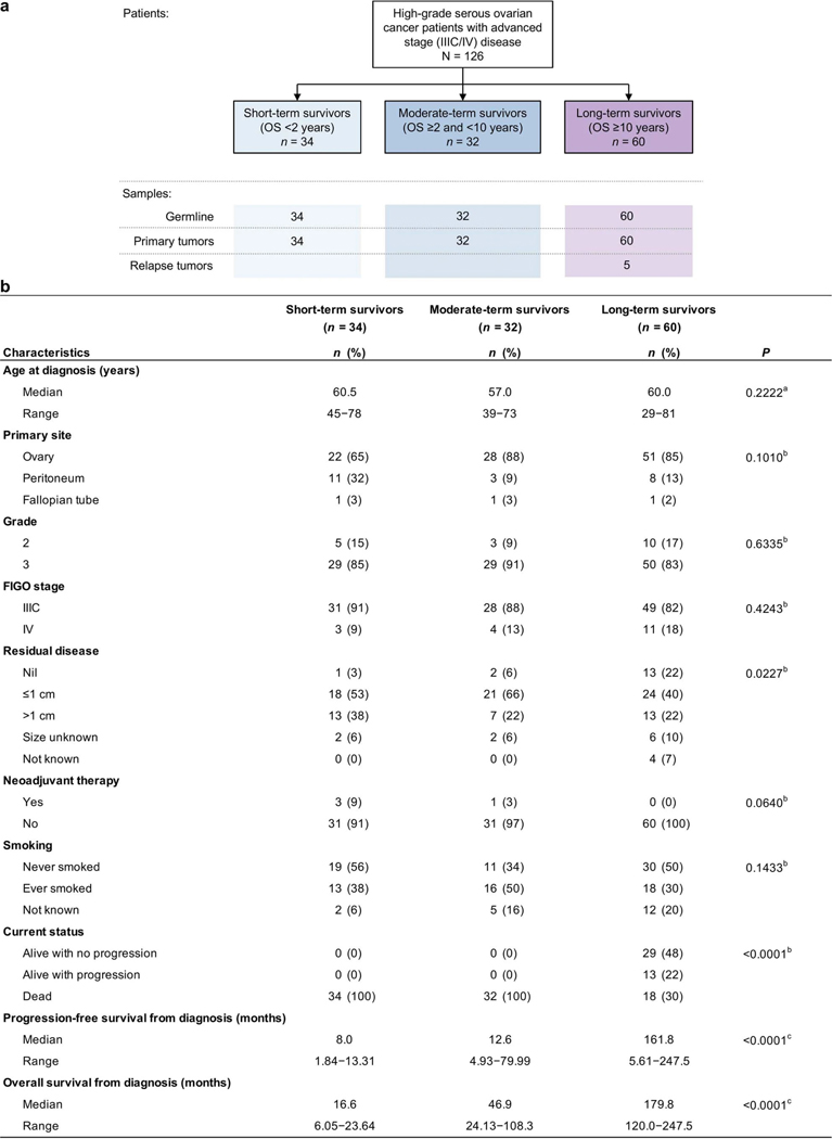
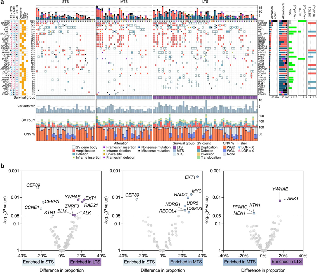
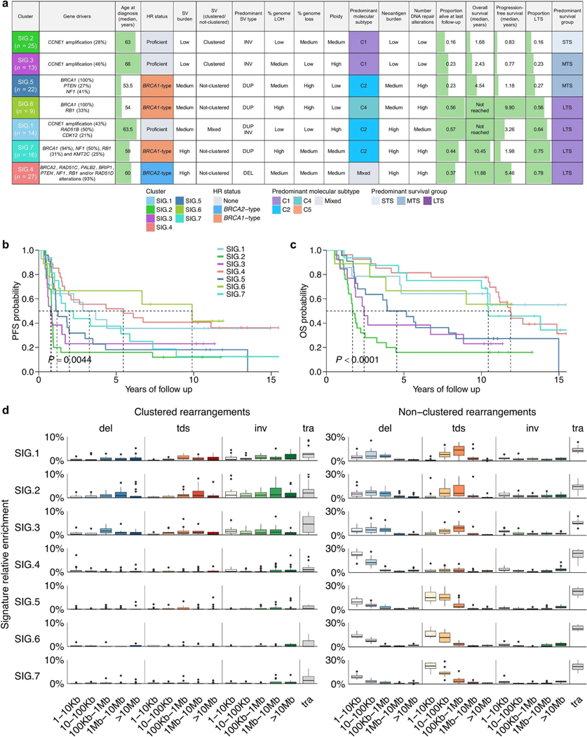
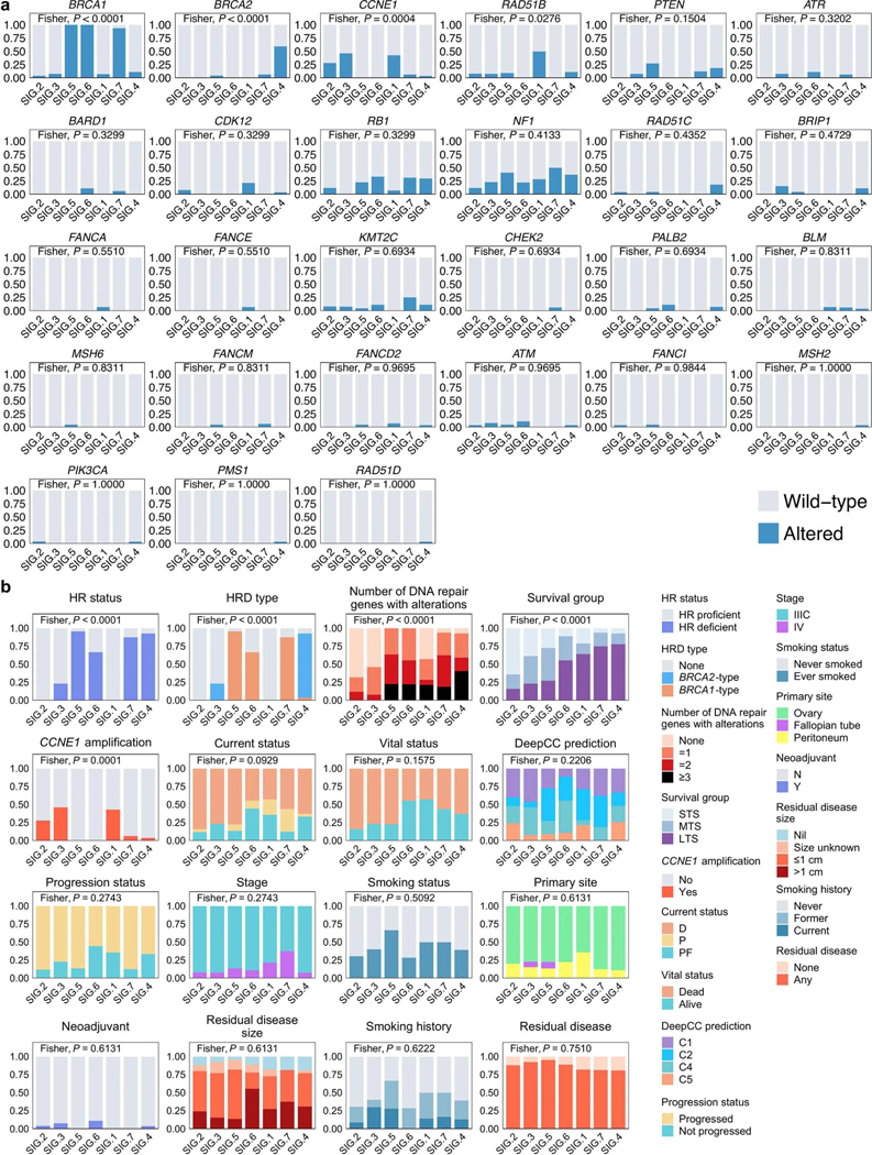
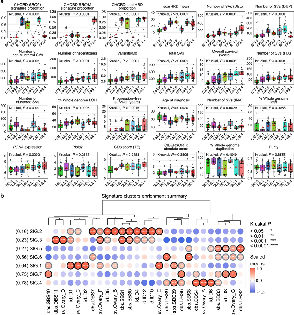
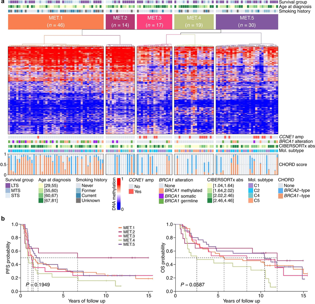
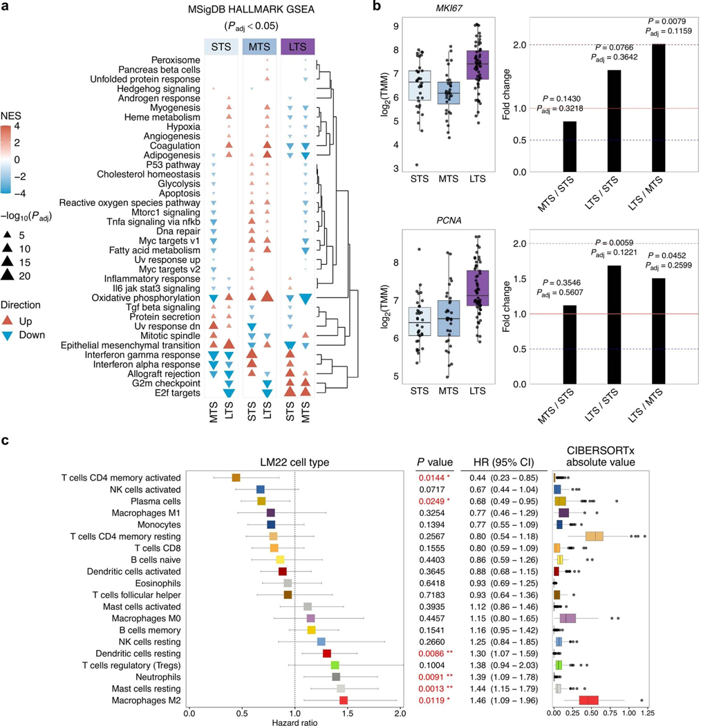
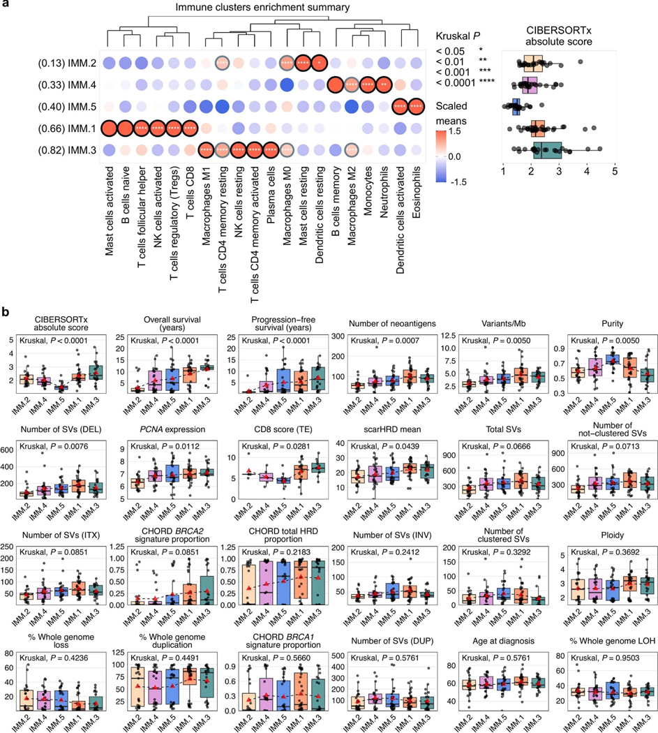
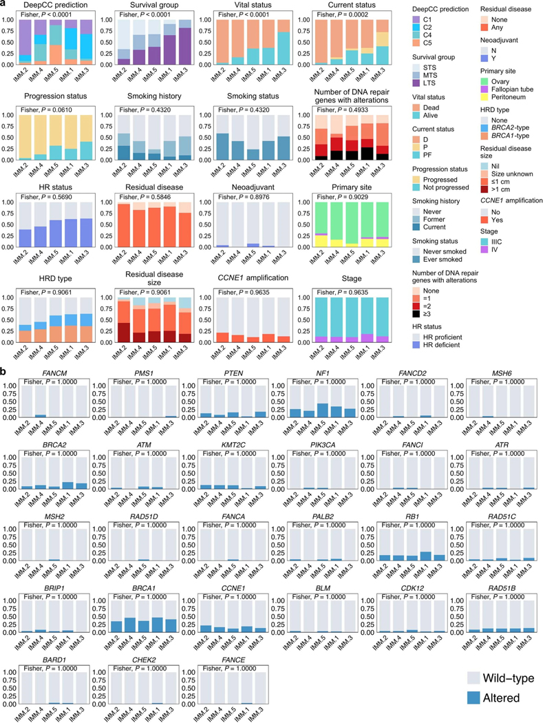
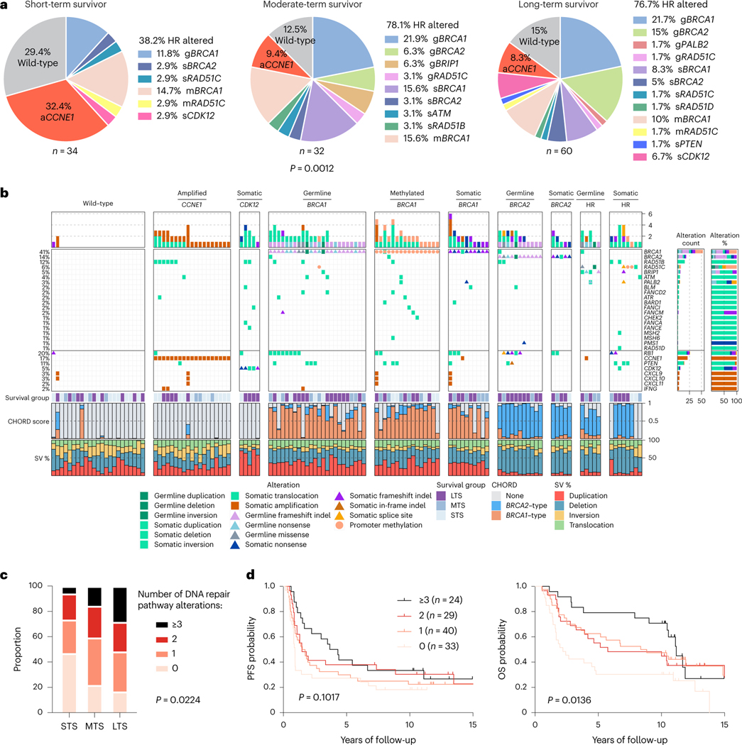
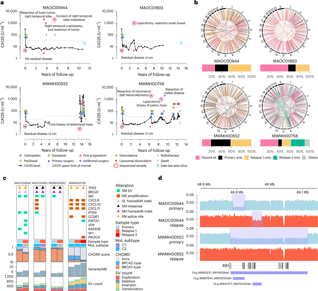
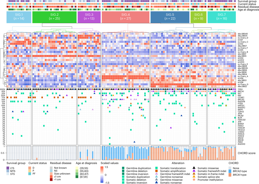
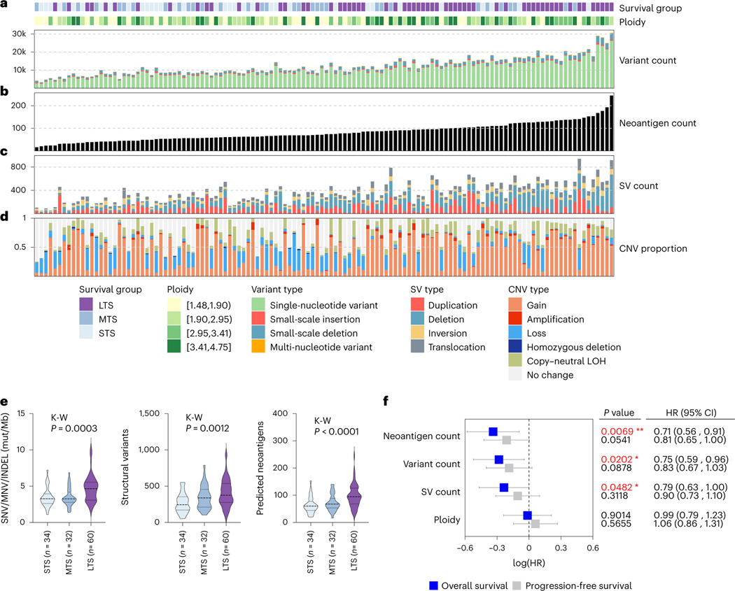
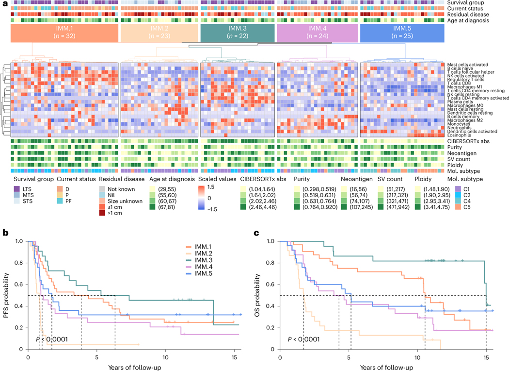
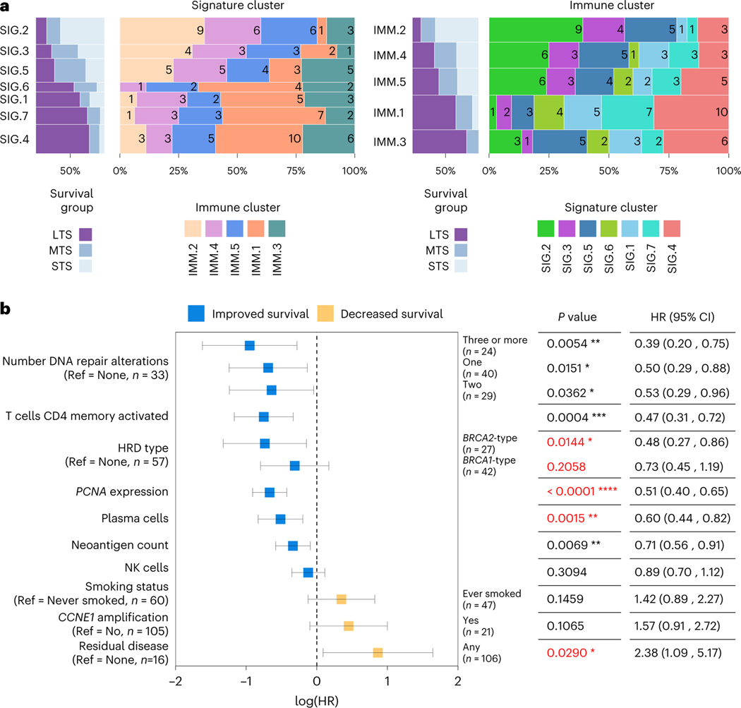
Fewer than half of all patients with advanced-stage high-grade serous ovarian cancers (HGSCs) survive more than five years after diagnosis, but those who have an exceptionally long survival could provide insights into tumor biology and therapeutic approaches. We analyzed 60 patients with advanced-stage HGSC who survived more than 10 years after diagnosis using whole-genome sequencing, transcriptome and methylome profiling of their primary tumor samples, comparing this data to 66 short- or moderate-term survivors. Tumors of long-term survivors were more likely to have multiple alterations in genes associated with DNA repair and more frequent somatic variants resulting in an increased predicted neoantigen load. Patients clustered into survival groups based on genomic and immune cell signatures, including three subsets of patients with BRCA1 alterations with distinctly different outcomes. Specific combinations of germline and somatic gene alterations, tumor cell phenotypes and differential immune responses appear to contribute to long-term survival in HGSC.

Extended Data Fig. 1:. Patient cohort.

a, Overview of patients (n = 126) and tumor samples analyzed in this study. In addition to paired germline and primary tumor samples in all patients, 5 relapse tumor samples were also analyzed from 4 long-term survivor patients. OS, overall survival. b, Clinical characteristics of patients by survival group. All patients received primary platinum therapy. ^aKruskal–Wallis, ^bChi-square, or ^clog-rank Mantel–Cox test P values comparing survival groups reported.

Extended Data Fig. 2:. Frequently altered cancer genes across survival groups.

a, Overview of somatic alterations in driver genes detected by GRIN, dNdScv, GISTIC, and/or in cancer-associated genes (COSMIC Cancer Gene Census) that are enriched in a survival group relative to another survival group. From left: two-sided Fisher’s test of the difference in proportions of altered samples between survival groups, triangles and color indicate direction of the log odds ratio (LOR; blue = down, pink = up), asterisks indicate P value < 0.05 (see Supplementary Table 6 for P values), P values were not adjusted for multiple comparisons; role of gene in COSMIC Cancer Gene Census (TSG, tumor suppressor gene); genomic alterations split by survival groups, bars at the top indicate the number of alterations in each listed gene per patient; bar plot of the number of samples with an alteration (alteration type indicated by color); bar plots showing the proportion of alteration types per gene; P values were calculated using the genomic random interval (GRIN) statistical model (one-sided) for recurrent structural variants (SV) (see Supplementary Data 2 for GRIN P values), the dNdScv likelihood-ratio test (two-sided) for recurrent base substitutions and small-scale deletions and insertions (see Supplementary Data 1 for dNdScv P values), and GISTIC2 permutation-of-markers test (one-sided) for recurrent copy-number variants (CNV) with red indicating amplification and blue indicating deletion (see Supplementary Data 3 for GISTIC2 P values), P values were adjusted for multiple comparisons using the Benjamini-Hochberg procedure (dNdScv, GISTIC2) or the robust false discovery rate procedure (GRIN) and are shown as negative log₁₀ P values and capped at 0.001 for display purposes. Each patient (column) is annotated with survival group (LTS, long-term survivor; MTS, moderate-term survivor; STS, short-term survivor). Below the alterations are bar plots indicating somatic mutation burden in variants per megabase (Mb); SV count including duplications, deletions, inversions and intrachromosomal rearrangements; and the proportion of the tumor genome that is duplicated (WGD) or lost (WGL). b, Pairwise comparison of the alteration frequencies between survival groups for genes in the COSMIC Cancer Gene Census. The difference in relative alteration frequency is shown on the x-axis and the P value (Fisher’s test, two-sided) is shown on the y-axis. Symbols of genes with P values < 0.05 are displayed. Multiple hypothesis correction was not applied in this analysis as adjusted P values were all greater than 0.1. Alterations in this analysis included non-synonymous mutations, homozygous deletions, amplifications and structural variants in coding genes that are expressed.

Extended Data Fig. 3:. Key features of mutational signature clusters and associated survival outcomes.

a, Summary of the key clinical and genomic features of each mutational signature cluster. Clusters are ordered top to bottom by lowest to highest proportion of long-term survivors (LTS) in each cluster. HR, homologous recombination; LOH, loss-of-heterozygosity; SV, structural variant; MTS, moderate-term survivor; STS, short-term survivor; DUP, duplications; DEL, deletions; INV, inversions. b, Kaplan–Meier analysis of progression-free and c, overall survival in patients stratified by signature clusters. P values calculated by Mantel–Cox log-rank test and dotted lines indicate median survival. d, Boxplots summarize the proportion (y-axis) of clustered and nonclustered rearrangements by size (x-axis) and type, for each mutational signature cluster (SIG.1 n = 14, SIG.2 n = 25, SIG.3 n = 13, SIG.4 n = 27, SIG.5 n = 22, SIG.6 n = 9, SIG.7 n = 16); boxes show the interquartile range (25–75th percentiles), central lines indicate the median, whiskers show the smallest/largest values within 1.5 times the interquartile range and values outside it are shown as individual data points. Del, deletions; tds, tandem duplications; inv, inversions, tra, interchromosomal translocations; Kb, kilobase; Mb, megabase.

Extended Data Fig. 4:. Categorical features of mutational signature clusters.

a, Proportion of patients affected by gene alterations per mutational signature cluster. Genes are ordered by significance using Fisher’s exact test (two-sided) and clusters are ordered by the proportion of long-term survivors. b, Proportion of patients with categorical features per cluster. Features are ordered by significance using Fisher’s exact test (two-sided) and the clusters are arranged by the proportion of long-term survivors. The Fisher’s test P values displayed in (a) and (b) are Benjamini-Hochberg adjusted P values. Features include homologous recombination (HR) status, homologous recombination deficiency (HRD) type, number of DNA repair pathway alterations, survival group (LTS, long-term survivor; MTS, moderate-term survivor; STS, short-term survivor), status at last follow-up (D, dead; P, progressed and alive; PF, progression-free and alive), self-reported smoking status, DeepCC molecular subtype (C1, mesenchymal; C2, immunoreactive; C4, differentiated; C5, proliferative), and neoadjuvant treatment (Y, yes; N, no).

Extended Data Fig. 5:. Clinical and genomic features of mutational signature clusters.

a, Boxplots summarize numerical, clinical and genomic features by mutational signature cluster; points represent each sample, boxes show the interquartile range (25–75th percentiles), central lines indicate the median, whiskers show the smallest/largest values within 1.5 times the interquartile range, red triangles indicate the mean, and dotted lines join the means of each cluster to visualize the trend. The Kruskal–Wallis test P values displayed are Benjamini-Hochberg adjusted P values. Features are ordered by their significance and clusters are ordered by the proportion of long-term survivors. CD8 scores were available for n = 54 primary tumors as previously measured by immunohistochemistry and scored as density of CD8+ T cells (average cells/mm², y axis) in the tumor epithelium (TE). HRD, homologous recombination deficiency; DEL, deletions; DUP; duplications; SV, structural variants; Mb, megabase; ITX, intrachromosomal rearrangements; LOH, loss-of-heterozygosity; INV, inversions. b, Bubble plot summary of mutational signature enrichment across signature clusters. The dendrogram is reused from the signature clustering (Fig. 3) to order the mutational signature types (columns). Mutational signature clusters (rows) are sorted by the proportion of long-term survivors in each cluster, indicated in brackets. The color and size of bubbles indicate the z-score scaled values of the mean signature exposure per cluster. Bubbles with a z-score of greater than or equal to 1 have a black border and bubbles with a z-score of greater than 0.5 but less than 1 have a gray border. Bordered bubbles have asterisks filled in to indicate Kruskal–Wallis test P values adjusted for multiple testing using Benjamini-Hochberg correction.

Extended Data Fig. 6:. DNA methylation clustering of primary tumor genomes.

a, Heatmap of methylation data following consensus clustering of primary tumors (columns) based on the standardized CpG probe intensities (M-values) of the 1% most variable CpG probes (rows; number of probes = 3,645) across all primary tumor samples (n = 126). The heatmap scale shows the beta values. Five methylation clusters were identified (MET.1–MET.5), and each patient (column) is annotated with survival group (LTS, long-term survivor; MTS, moderate-term survivor; STS, short-term survivor), age at diagnosis (quartiles), and self-reported smoking history. Tumor samples are also classified according to CCNE1 amplification (amp) status, BRCA1 alteration status, CIBERSORTx absolute (abs) immune scores (quartiles), and molecular subtype (C1, mesenchymal; C2, immunoreactive; C4, differentiated; C5, proliferative). Bars in the bottom panel represent the BRCA1 (orange) and BRCA2 (blue) type homologous recombination deficiency (CHORD) scores of each tumor sample. b, Kaplan–Meier analysis of progression-free (PFS) and overall survival (OS) in patients stratified by methylation clusters. P values calculated by Mantel–Cox log-rank test and dotted lines indicate median survival in years since diagnosis.

Extended Data Fig. 7:. Transcriptional phenotypes in long-term survivors.

a, Clustered heatmap summarizing gene set enrichment analysis (GSEA) using the hallmark Molecular Signatures Database (MSigDB) gene sets. Direction and color of triangles relate to the normalized enrichment score (NES) as generated by FGSEA. P values (two-sided) were calculated using the FGSEA default Monte Carlo method; the size of the triangles corresponds to the negative log₁₀ Benjamini-Hochberg adjusted P value (P_adj). The columns are split by survival groups (STS, short-term survivor; MTS, moderate-term survivor; LTS, long-term survivor), with the direction of enrichment denoted by the group in the heading (numerator) versus the two other groups labeled below. b, Boxplots summarize expression of MKI67 and PCNA proliferation gene markers across the survival groups (left; STS n = 34, MTS n = 32, LTS n = 60); points represent each sample, boxes show the interquartile range (25–75th percentiles), central lines indicate the median, and whiskers show the smallest/largest values within 1.5 times the interquartile range. Differential expression analysis was performed using DESeq2 to determine fold change (right) of gene expression between survival groups (two-tailed Wald test, both unadjusted P values and Benjamini-Hochberg adjusted P values (P_adj) are shown). c, Forest plot (left) indicates the hazard ratio (HR, squares) and 95% confidence interval (CI; whiskers) for overall survival calculated using a univariate Cox proportional hazard regression model based on the LM22 immune cell types detected by CIBERSORTx analysis (n = 126 patients). Cell types are arranged by HR. P values < 0.05 are colored red (*P < 0.05, **P < 0.01) and were not adjusted for multiple comparisons. Absolute enrichment scores per cell type across the cohort are shown in boxplots (right); boxes show the interquartile range (25–75th percentiles), central lines indicate the median, whiskers show the smallest/largest values within 1.5 times the interquartile range and values outside it are shown as individual data points.

Extended Data Fig. 8:. Genomic and clinical features of immune clusters.

a, A condensed bubble plot of the various LM22 cell types used for the immune clustering (IMM.1 n = 32, IMM.2 n = 23, IMM.3 n = 22, IMM.4 n = 24, IMM.5 n = 25). The dendrogram is reused from the immune clustering (Fig. 5a) to order the cell types. Immune clusters (rows) are sorted by the proportion of long-term survivors indicated in brackets. The color and size of bubbles indicate z-score scaled values of the mean abundance of cell types per cluster. Bubbles with a z-score of greater than or equal to 1 have a black border, and those with a z-score of greater than 0.5 but less than 1 have a gray border. Asterisks indicate Kruskal–Wallis test P values adjusted for multiple testing using Benjamini-Hochberg correction. Boxplots (right) summarize CIBERSORTx absolute scores of each cluster; points represent each sample, boxes show the interquartile range (25–75th percentiles), central lines indicate the median, and whiskers show the smallest/largest values within 1.5 times the interquartile range. b, Boxplots summarize numerical, clinical and genomic features by immune cluster (IMM.1 n = 32, IMM.2 n = 23, IMM.3 n = 22, IMM.4 n = 24, IMM.5 n = 25); points represent each sample, boxes show the interquartile range (25–75th percentiles), central lines indicate the median, whiskers show the smallest/largest values within 1.5 times the interquartile range, red triangles indicate the mean, and dotted lines join the means of each cluster to visualize the trend. The Kruskal–Wallis test P values displayed are Benjamini-Hochberg adjusted. Features are ordered by their significance and clusters are ordered by the proportion of long-term survivors. CD8 scores were available for n = 54 primary tumors as previously measured by immunohistochemistry and scored as density of CD8+ T cells (average cells/mm², y axis) in the tumor epithelium (TE). HRD, homologous recombination deficiency; DEL, deletions; DUP; duplications; SV, structural variants; Mb, megabase; ITX, intrachromosomal rearrangements; LOH, loss-of-heterozygosity; INV, inversions.

Extended Data Fig. 9:. Categorical features of immune clusters.

a, Proportion of patients with categorical features per cluster. Features are ordered by significance using Fisher’s exact test (two-sided) and the clusters are arranged by the proportion of long-term survivors. Features include homologous recombination (HR) status, homologous recombination deficiency (HRD) type, number of DNA repair pathway alterations, survival group (LTS, long-term survivor; MTS, moderate-term survivor; STS, short-term survivor), status at last follow-up (D, dead; P, progressed and alive; PF, progression-free and alive), self-reported smoking status, DeepCC molecular subtype (C1, mesenchymal; C2, immunoreactive; C4, differentiated; C5, proliferative), and neoadjuvant treatment (Y, yes; N, no). b, Proportion of patients affected by gene alterations per immune cluster. Genes are ordered by significance using Fisher’s exact test (two-sided) and clusters are ordered by the proportion of long-term survivors. The Fisher’s test P values displayed in (a) and (b) are Benjamini-Hochberg adjusted P values.

Fig. 1 |. HGSCs with multiple altered DNA repair pathway genes are associated with long-term survival.

a, Proportion of patients affected by homologous recombination (HR) DNA repair pathway gene alterations and CCNE1 gene amplification (aCCNE1) in each survival group. Homologous recombination alterations include pathogenic germline (g) or somatic (s) mutations, and BRCA1 or RAD51C promoter methylation (m) as indicated. One alteration is counted for patients with more than one change, prioritizing alterations by variant allele frequency and/or by evidence of genomic scarring associated with the candidate driver alteration. Differences in proportions of homologous recombination-altered, CCNE1 amplified and wild-type tumors between survival groups were assessed by chi-square. b, Bars at the top represent the number of alterations in each listed gene per patient. Pathogenic germline and somatic alterations in homologous recombination pathway genes are shown, as well as alterations in other DNA repair associated genes, immune genes and CCNE1. Each patient (column) is annotated with survival group (LTS, long-term survivor; MTS, moderate-term survivor; STS, short-term survivor). Bars indicate the level of homologous recombination deficiency (HRD) in each primary tumor sample, measured as probabilities of BRCA1-type (orange) HRD, BRCA2-type(blue) HRD, or homologous recombination proficiency (none, gray), as predicted by CHORD. Bar plots at the bottom indicate the proportion of total detected structural variants (SV) classified as duplications, deletions, inversions or interchromosomal translocations. Samples are grouped by the primary gene alteration identified in each patient. Alteration count and proportion of alteration types per gene are shown as bar plots on the right. c, Proportion of patients with 0, 1, 2 or 3 or more DNA repair pathway alterations by survival group (LTS, long-term survivor; MTS, moderate-term survivor; STS, short-term survivor). Differences in proportions between groups were assessed by chi-square. d, Kaplan-Meier analysis of progression-free survival (PFS) (left) and OS in patients (right) with 0, 1, 2 or 3 or more DNA repair pathway alterations. P values calculated by Mantel-Cox log-rank test.

Fig. 2 |. Genomic analysis of matched primary and recurrent HGSC in four long-term survivors.

a, Serum CA125 levels (solid black lines) on a log scale (y axis) of long-term survivor relapse cases (n = 4), measured at various intervals over time (x axis). The upper limit of normal for CA125 (dotted gray lines) can vary depending on the CA125 assay performed. Colored circles and rectangles represent different lines of treatment as indicated. All patients were diagnosed with stage IIIC HGSC at primary surgery (blue triangle). Also indicated is the time of first progression (red triangle), additional surgeries (purple asterisks), sequenced sample (red ring), death (gray cross) or date last seen alive (green diamond). b, Circos plots summarize the structural variants (lines) that are shared or unique between primary and relapse samples for each case as indicated. Bar plots below show the proportion of total shared and unique structural variants (SVs) in each patient. In the patient with two relapse samples, structural variants that were shared only by two tumor samples were classified as “others”. c, Somatic (SM) and germline (GL) alterations in primary and relapse tumor samples in genes of interest (rows). Each sample (column) is annotated with sample type (primary or relapse) and molecular (Mol.) subtype if RNA was available. Bars indicate the level of HRD in each tumor sample, measured as probabilities of BRCA1-type(orange) HRD, BRCA2-type(blue) HRD, or homologous recombination proficient (none, gray), as predicted by CHORD. Bar plots at the bottom indicate somatic mutation burden in variants per megabase (Mb) and SV counts in each sample. d, BigWig tracks of DNA sequencing coverage (y axis) in two paired primary (shaded blue) and relapse (shaded red) tumor samples showing the locations (x axis) of deletions (blue rectangles) identified in RB1.

Fig. 3 |. Long-term survivor tumor genomes are characterized by distinct molecular phenotypes.

Heatmap of mutational signatures following consensus clustering based on proportions of mutational signature exposures in each primary tumor sample (n = 126). Patient (column) scaled z-scores are shown in the heatmap. Seven mutational signature clusters were identified (SIG.1-SIG.7), and each patient (column) is annotated with survival group (LTS, long-term survivor; MTS, moderate-term survivor; STS, short-term survivor), status at last follow-up (D, dead; P, progressed and alive; PF, progression-free and alive), residual disease and age at diagnosis (in years; quartiles). Bars represent the BRCA1-type (orange) and BRCA2-type (blue) HRD (CHORD) scores of each tumor sample, and germline and somatic alterations affecting genes of interest are shown in the bottom panel.

Fig. 4 |. Elevated somatic mutation burden in long-term survivors.

a, Bars indicate the total variant count of each primary tumor sample (n = 126), including SNVs, small-scale insertions and deletions (INDELs) and multinucleotide variants (MNVs). b, Tumor samples are ordered left to right from fewest to largest number of neoantigens (black bars). c, Bars indicate total number of large-scale structural variants (SVs) in primary tumors, including duplications, deletions, inversions and interchromosomal translocations. d, Bars indicate the proportion of each tumor genome affected by CNVs, including regions of gain, amplification, loss, homozygous deletion and copy-neutral loss of heterozygosity (LOH). e, Violin plots represent the tumor mutation burden, structural variant count and predicted neoantigen counts of tumor genomes in each survival group. Dashed lines represent the median and dotted lines represent the lower and upper quartiles. Kruskal-Wallis (K-W) test P values are reported. STS, short-term survivor; MTS, moderate-term survivor; LTS, long-term survivor; mut/Mb, mutations per megabase. f, Forest plot indicates the HR (squares) and 95% Cl (whiskers) for progression-free and OS (n = 126 patients) calculated using a univariate Cox proportional hazard regression model based on genomic features as indicated; P values < 0.05 are colored red (*P < 0.05, **P < 0.01) and were not adjusted for multiple comparisons.

Fig. 5 |. Immune phenotypes of long-term survivors.

a, Heatmap of scaled abundance of immune cell types following consensus clustering based on CIBERSORTx estimated absolute abundance of immune cell types from bulk RNA-seq data of each primary tumor (n = 126). Five immune clusters were identified (IMM.1-IMM.5), and each patient (column) is annotated with survival group (LTS, long-term survivor; MTS, moderate-term survivor; STS, short-term survivor), status at last follow-up (D, dead; P, progressed and alive; PF, progression-free and alive), residual disease size and age at diagnosis (quartiles). CIBERSORTx absolute (abs) immune scores, tumor purity, neoantigen counts, structural variant (SV) counts and ploidy estimates are shown as quartiles. Tumor samples are also classified according to molecular subtype (Cl, mesenchymal; C2, immunoreactive; C4, differentiated; C5, proliferative). b,c, Kaplan-Meier analysis of progression-free survival (b) and OS (c) in patients stratified by immune clusters. P values were calculated by Mantel-Cox log-rank test, and dotted lines indicate median survival.

Fig. 6 |. Key features associated with exceptional survival in HGSC.

a, Spine plots showing the proportion of samples shared between the mutational signature clusters (left) and the immune clusters (right), with the number of overlapping samples indicated inside the colored bars. Also shown is the proportion of survival groups (STS, short-term survivor; MTS, moderate-term survivor; LTS, long-term survivor) in each cluster. Each of the two types of clusters is ordered horizontally and vertically by the overall proportion of LTS. The height of the bars indicates the number of samples in the cluster. b, Forest plot illustrates the HR (squares) and 95% CI (whiskers) for OS calculated using a univariate Cox proportional hazard regression model based on selected features; results were not adjusted for multiple comparisons (*P < 0.05, **P < 0.01, ***P < 0.001, ****P < 0.0001). Features are sorted top to bottom by smallest to largest HR and P values less than 0.05 in multivariable model are colored red. Complete univariable and multivariable results, including feature associations with progression-free survival, are provided in Supplementary Tables 13, 14. Ref indicates the reference used for categorical features, and n indicates the number of samples in the categorical group.

References

1. Millstein J. et al. Prognostic gene expression signature for high-grade serous ovarian cancer. Ann. Oncol 31, 1240–1250 (2020). - PMC - PubMed
1. Hoppenot C, Eckert MA, Tienda SM & Lengyel E. Who are the long-term survivors of high grade serous ovarian cancer? Gynecol. Oncol 148, 204–212 (2018). - PubMed
1. Fago-Olsen CL et al. Does neoadjuvant chemotherapy impair long-term survival for ovarian cancer patients? A nationwide Danish study. Gynecol. Oncol 132, 292–298 (2014). - PubMed
1. Chi DS et al. What is the optimal goal of primary cytoreductive surgery for bulky stage IIIC epithelial ovarian carcinoma (EOC)? Gynecol. Oncol 103, 559–564 (2006). - PubMed
1. Horowitz NS et al. Does aggressive surgery improve outcomes? Interaction between preoperative disease burden and complex surgery in patients with advanced-stage ovarian cancer: an analysis of GOG 182. J. Clin. Oncol 33, 937–943 (2015). - PMC - PubMed
Publication types