Data-driven discovery of canonical large-scale brain dynamics

Abstract

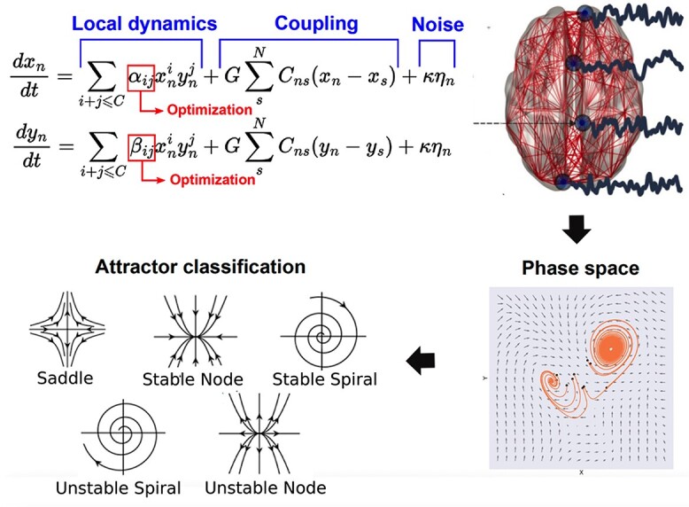
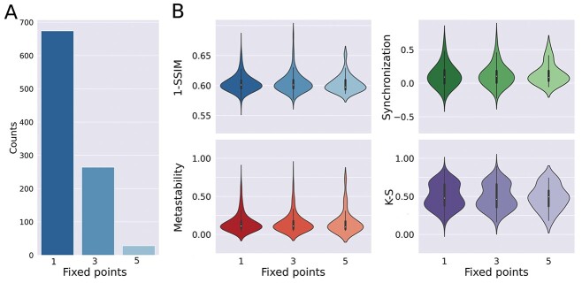
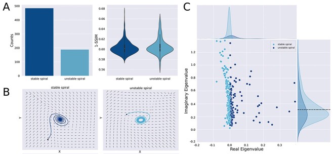
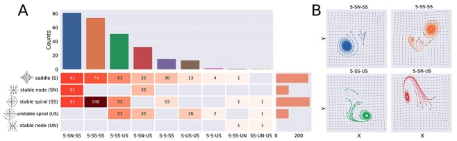
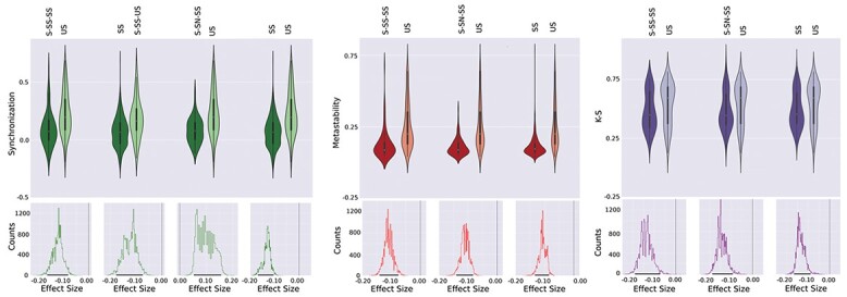
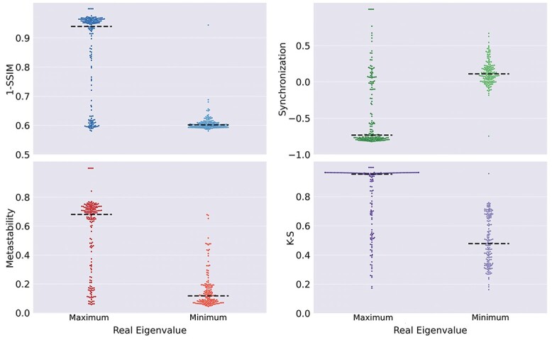
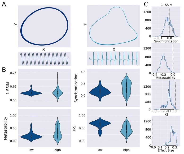
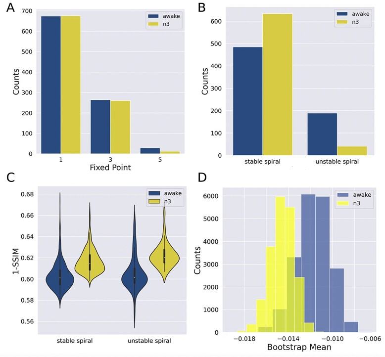
Human behavior and cognitive function correlate with complex patterns of spatio-temporal brain dynamics, which can be simulated using computational models with different degrees of biophysical realism. We used a data-driven optimization algorithm to determine and classify the types of local dynamics that enable the reproduction of different observables derived from functional magnetic resonance recordings. The phase space analysis of the resulting equations revealed a predominance of stable spiral attractors, which optimized the similarity to the empirical data in terms of the synchronization, metastability, and functional connectivity dynamics. For stable limit cycles, departures from harmonic oscillations improved the fit in terms of functional connectivity dynamics. Eigenvalue analyses showed that proximity to a bifurcation improved the accuracy of the simulation for wakefulness, whereas deep sleep was associated with increased stability. Our results provide testable predictions that constrain the landscape of suitable biophysical models, while supporting noise-driven dynamics close to a bifurcation as a canonical mechanism underlying the complex fluctuations that characterize endogenous brain activity.

Keywords: brain dynamics; computational modeling; fMRI; resting state; sleep.

Fig. 1

Procedure followed for the data-driven discovery of canonical whole-brain dynamics. Each iteration of the model consisted in local dynamics given by the 2 variables x, y combined in polynomial terms up to degree C with coefficients α_ij, coupling by the connectome scaled by G, and noise scaled by κ. After the initial selection of G, the parameters α_ij were optimized to reproduce the fMRI functional connectivity (FC) between all pairs of nodes. The optimal local dynamics can be characterized in terms of the 2D phase space of variables x, y, where different attractors can be identified and used to characterize the resulting dynamics.

Fig. 2

Local dynamics tend to exhibit a single fixed-point, and the similarity between simulated and empirical dynamics is independent of the number of fixed-points. A) Number of iterations resulting in 1, 3, and 5 fixed-points. B) Four different metrics computed after separating the solutions by the number of fixed-points in the phase space. No differences were encountered when comparing local dynamics with different numbers of fixed-points.

Fig. 3

Stable spirals are most prevalent for local dynamics with one isolated fixed-point. A) Left panel: Number of iterations resulting in local dynamics with stable and unstable spirals. Right panel: 1-SSIM for both types of local dynamics. B) Examples of phase spaces with each type of local dynamics. Note that the unstable spiral is surrounded by a limit cycle (attractor consisting of a periodic trajectory). C) Scatter plot of the imaginary vs. real eigenvalues of the fixed-point, where each point corresponds to an independent iteration of the model. The vertical line of null real eigenvalues determines the stability of the spiraling solution.

Fig. 4

Saddle nodes and stable spirals are the most predominant for local dynamics with 3 fixed-points. A) Matrix entries indicate the total number of fixed-points (rows) that are present in a specific combination (columns). The bar plot in the upper panel shows the number of solutions found for each combination of 3 fixed-points, whereas the bars of the right count the number of individual fixed-points, regardless of their combinations. B) Phase space plots of the 4 most predominant combinations of fixed-points. The black points indicate the random values used for initializing the simulation.

Fig. 5

Local dynamics with stable spirals resulted in better reproduction of the empirical data in terms of synchronization, metastability, and Kolmogorov–Smirnov distance between distributions of FCD values. Violin plots present the distribution of performance metrics for all solutions with the local dynamics indicated by the labels. The bottom panels show the distribution of effect sizes obtained using bootstrap. The vertical line indicates zero, i.e. null effect size, whereas the 95% confidence intervals are indicated using thick black lines in the x-axis.

Fig. 6

Spiral fixed-points with real eigenvalues closer to zero resulted in a better reproduction of the empirical observables regardless of the type of fixed-point. Comparison of the goodness of fit in terms of 4 different metrics for the spirals with maximum vs. minimum real eigenvalue. The black dashed lines denote the median of each distribution.

Fig. 7

The anharmonicity of stable limit cycles in the local dynamics influenced the goodness of fit according to different metrics. A) Examples of stable limit cycles and time series of high (right) and low (left) anharmonicity. B) Violin plots summarizing the distribution of the performance metrics for all solutions presenting stable limit cycles of low and high anharmonicity. C. Distribution of effect sizes for the difference in the performance metrics obtained using bootstrap. The vertical line indicates zero, i.e. null effect size, whereas the 95% confidence intervals are indicated using thick black lines in the x-axis.

Fig. 8

Deep sleep resulted in the stabilization of fMRI dynamics. A) Number of fixed-points in the optimal local dynamics, for wakefulness and n3. B) Relative prevalence of stable spirals vs. unstable spirals for both brain states. C) Distance to the empirical data (1-SSIM) for wakefulness and n3 sleep. D) Histogram of the real eigenvalues of the stable spiral fixed-points computed using a bootstrap procedure and for both brain states. The shift towards left for n3 indicates increased stability of the local dynamics relative to wakefulness.

References

1. Acebrón J, Bonilla LL, Pérez Vicente CJ, Ritort F, Spigler R. The Kuramoto model: a simple paradigm for synchronization phenomena. Rev Mod Phys. 2005:77(1):137–185. 10.1103/RevModPhys.77.137. - DOI
1. Bassett DS, Gazzaniga MS. Understanding complexity in the human brain. Trends Cogn Sci. 2011:15(5):200–209. 10.1016/j.tics.2011.03.006. - DOI - PMC - PubMed
1. Buendía V, di Santo S, Villegas P, Burioni R, Muñoz M. Self-organized bistability and its possible relevance for brain dynamics. Physical Review Research. 2020:2(1):013318. 10.1103/PhysRevResearch.2.013318. - DOI
1. Bullmore E, Sporns O. Complex brain networks: graph theoretical analysis of structural and functional systems. Nat Rev Neurosci. 2009:10(3):186–198. 10.1038/nrn2575. - DOI - PubMed
1. Chialvo DR. Emergent complex neural dynamics. Nat Phys. 2010:6(10):744–750. 10.1038/nphys1803. - DOI
LinkOut - more resources