Investigating the effect of oblique image acquisition on the accuracy of QSM and a robust tilt correction method

Abstract

Purpose: Quantitative susceptibility mapping (QSM) is used increasingly for clinical research where oblique image acquisition is commonplace, but its effects on QSM accuracy are not well understood.

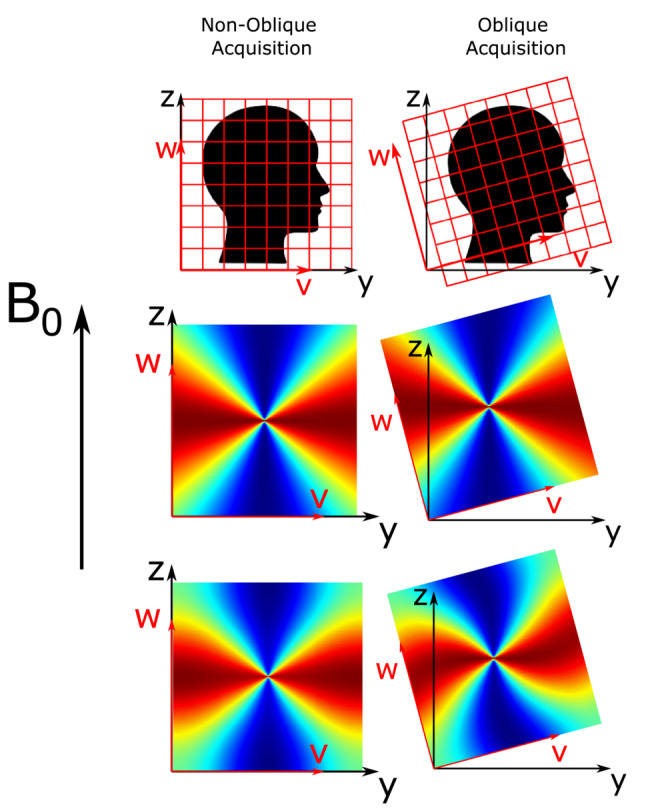
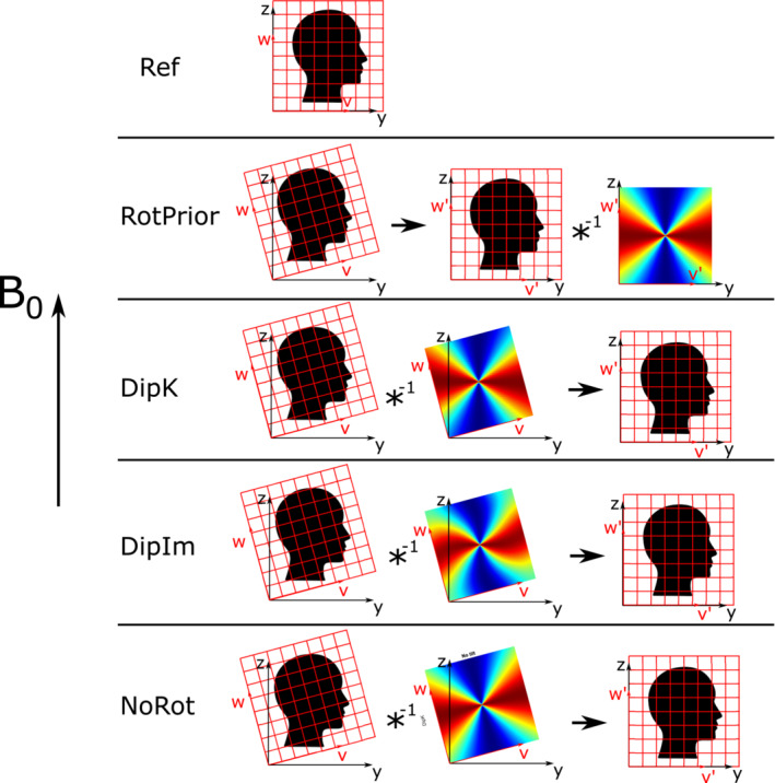
Theory and methods: The QSM processing pipeline involves defining the unit magnetic dipole kernel, which requires knowledge of the direction of the main magnetic field ${\hat{B}}_0$ with respect to the acquired image volume axes. The direction of ${\hat{B}}_0$ is dependent on the axis and angle of rotation in oblique acquisition. Using both a numerical brain phantom and in vivo acquisitions in 5 healthy volunteers, we analyzed the effects of oblique acquisition on magnetic susceptibility maps. We compared three tilt-correction schemes at each step in the QSM pipeline: phase unwrapping, background field removal and susceptibility calculation, using the RMS error and QSM-tuned structural similarity index.

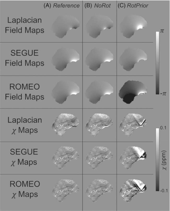
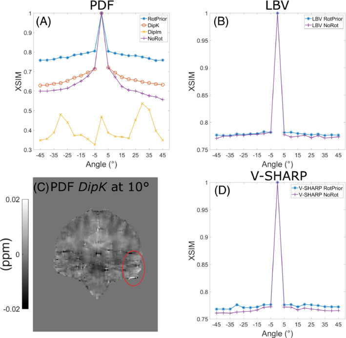
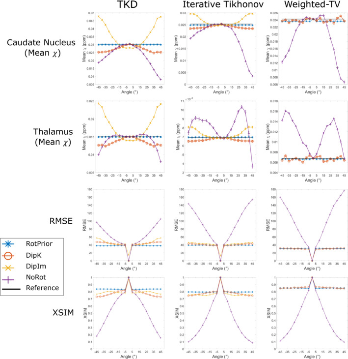
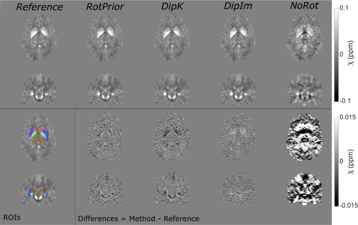
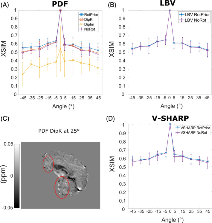
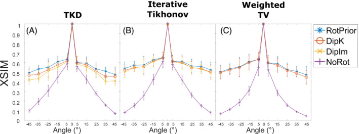
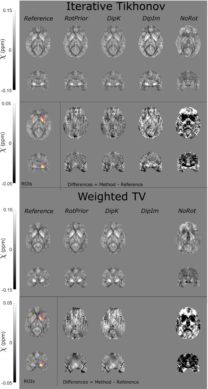
Results: Rotation of wrapped phase images gave severe artifacts. Background field removal with projection onto dipole fields gave the most accurate susceptibilities when the field map was first rotated into alignment with ${\hat{B}}_0$ . Laplacian boundary value and variable-kernel sophisticated harmonic artifact reduction for phase data background field removal methods gave accurate results without tilt correction. For susceptibility calculation, thresholded k-space division, iterative Tikhonov regularization, and weighted linear total variation regularization, all performed most accurately when local field maps were rotated into alignment with ${\hat{B}}_0$ before susceptibility calculation.

Conclusion: For accurate QSM, oblique acquisition must be taken into account. Rotation of images into alignment with ${\hat{B}}_0$ should be carried out after phase unwrapping and before background-field removal. We provide open-source tilt-correction code to incorporate easily into existing pipelines: https://github.com/o-snow/QSM_TiltCorrection.git.

Keywords: QSM; QSM accuracy; electromagnetic tissue properties; oblique acquisition; quantitative susceptibility mapping; tilted slices.

FIGURE 1

Nonoblique and oblique acquisition about the $\mathrm{x}$‐axis ($\mathrm{u}$‐axis) of axial slices (top row) with corresponding k‐space dipoles (middle row) and image‐space dipoles (bottom row). The image axes $(\mathrm{u},\mathrm{v},\mathrm{w})$ and scanner axes $(\mathrm{x},\mathrm{y},\mathrm{z})$ are shown in red and black, respectively. Note that the rotation axis is at the center of the image

FIGURE 2

All tilt‐correction schemes including the reference, nonoblique acquisition for rotations about the x‐axis. The native (oblique) image space $(\widehat{u},\widehat{v},\widehat{w})$ was transformed to $(\widehat{u^{\prime }},\widehat{v^{\prime }},\widehat{w^{\prime }}),$ aligned with the scanner frame. The black arrow denotes rotation into the scanner frame of reference. DipK, DipIm, and NoRot were rotated back into the reference (scanner) frame after correction to facilitate comparisons. RotPrior and NoRot still apply when no dipole is used

FIGURE 3

Method for calculating the synthetic background field from a head‐shaped susceptibility map obtained by thresholding the numerical phantom magnitude image and a pseudo‐CT image to delineate soft tissue and bone, respectively. The thresholded magnitude and pseudo‐CT images were filtered for smoothness using a 3 × 3 × 3 box filter

FIGURE 4

Effect of tilt correction before phase unwrapping in the numerical phantom. Phase‐unwrapped field maps and the resulting susceptibility maps at 15° for the NoRot (column b) and RotPrior (column c) tilt‐correction methods relative to the reference (column a). Rotation of the wrapped field maps before phase unwrapping with Laplacian, SEGUE, and ROMEO techniques results in errors along phase wraps and incorrect unwrapping, leading to prominent artifacts in the final susceptibility maps

FIGURE 5

Effect of different tilt‐correction schemes on QSM with three background field removal methods in a numerical phantom. Susceptibility maps for QSM‐tuned structural similarity index (XSIM) comparisons were calculated with iterative Tikhonov regularization. For projection onto dipole fields (PDF) (A), the XSIM metric shows that RotPrior gives the most accurate susceptibilities, with DipIm performing the worst. When using PDF with DipK, striping artifacts (C, red ellipse) arise in the local field maps for tilted acquisitions. Laplacian boundary value (LBV) and variable‐kernel sophisticated harmonic artifact reduction for phase data (V‐SHARP) (C,D) are shown to be largely unaffected by oblique acquisition with differences arising primarily from rotation interpolations

FIGURE 6

Mean susceptibilities in the caudate and thalamus (top rows), and XSIM (bottom row) across all tilt angles for all tilt‐correction schemes, plus all three $\chi$ calculation methods in the numerical phantom. The RMS error (RMSE) measurements shown in Supporting Information Figure S4 agree with the XSIM findings. NoRot performs worst across all angles. RotPrior is the most accurate tilt‐correction scheme. For weighted linear total variation (TV), DipK and RotPrior have similar XSIM values but the mean thalamus $\chi$ varies more over angles with DipK. Note that DipIm is not shown for weighted linear TV, as this method fails

FIGURE 7

χ maps and difference images illustrating the effects of all tilt correction schemes in the numerical phantom. An axial and a coronal slice are shown for a volume tilted at 25° and a reference 0° volume with all χ maps calculated using the iterative Tikhonov method. The ROIs analysed are also shown (bottom left). RotPrior performs the best while NoRot results in substantial χ errors across the whole brain. The results from TKD and weighted linear TV (not shown) are very similar

FIGURE 8

Effect of different tilt‐correction schemes on background field removal in vivo. The average XSIM measurements across all subjects were used to compare the $\chi$ maps calculated with iterative Tikhonov regularization after background field removal to the nonoblique (0°) reference map. The PDF method (A) has the highest XSIM with RotPrior and the lowest XSIM with DipIm, followed by NoRot, confirming the results in the numerical phantom (Figure 5). Striping artifacts are found in local field maps when using DipK and PDF (C, red ellipses) but are obscured after rotation and registration back into the reference 0° space due to interpolation. The LBV (B) and V‐SHARP (D) methods are shown to be unaffected by oblique acquisition in vivo as well as in the numerical phantom (Figure 5B and 5D). Error bars represent the SD of the mean XSIM across subjects

FIGURE 9

Average XSIM plots over all angles for all tilt‐correction schemes and all three $\chi$ calculation methods across all subjects in vivo. The RMSE measurements in Supporting Information Figure S4 agree with these XSIM findings. These results are similar to those in the numerical phantom (Figure 3), with RotPrior consistently reporting higher XSIM measures than other methods and NoRot performing worst across all methods. At nonzero tilt angles, XSIM has a respectively high/low baseline level arising from rotation and registration interpolations. DipIm fails for weighted linear TV, and therefore is omitted from the plots in the last column. Error bars represent the SD of the mean XSIM across subjects

FIGURE 10

The χ maps and difference images illustrating the effects of all tilt‐correction schemes on susceptibility calculation in vivo. An axial and a coronal slice are shown for a volume tilted at 45° and a reference (0°) volume with all χ maps calculated using the iterative Tikhonov method (top) and weighted linear TV (bottom). Weighted linear TV with DipIm fails at nonzero angles and is therefore omitted from the figure. NoRot leads to the largest differences and image artifacts throughout the brain for iterative Tikhonov and weighted linear TV methods. The EVE ROIs used are shown (bottom left). Results from TKD (Supporting Information Figure S6) are very similar

References

-
- Jack CR, Theodore WH, Cook M, McCarthy G. MRI‐based hippocampal volumetrics: data acquisition, normal ranges, and optimal protocol. Magn Reson Imaging. 1995;13:1057‐1064. - PubMed
- Chen W, Zhu XH. Suppression of physiological eye movement artifacts in functional MRI using slab presaturation. Magn Reson Med. 1997;38:546‐550. - PubMed
- Deistung A, Schweser F, Reichenbach JR. Overview of quantitative susceptibility mapping. NMR Biomed. 2017;30:e3569. - PubMed
Publication types
MeSH terms
Grants and funding
LinkOut - more resources
Full Text Sources