Spatial-ID: a cell typing method for spatially resolved transcriptomics via transfer learning and spatial embedding

Abstract

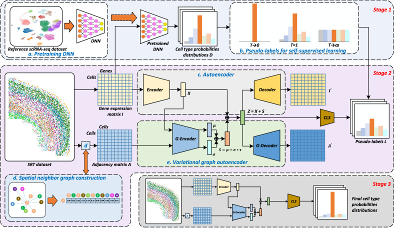
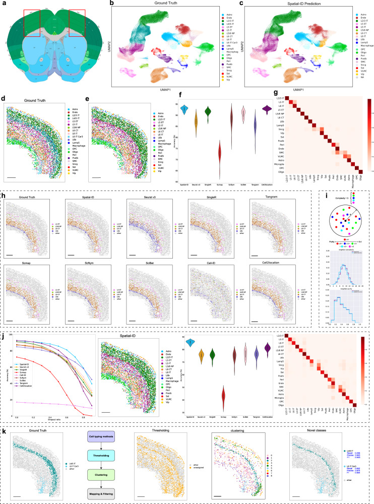
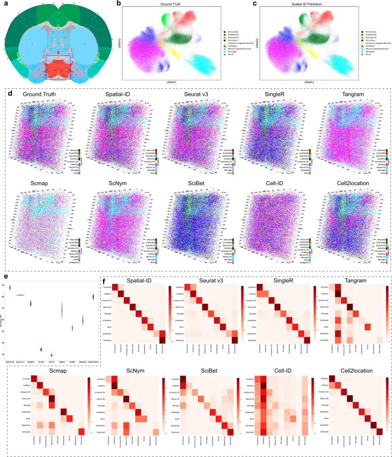
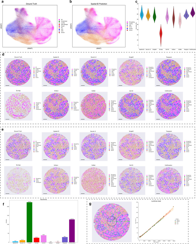
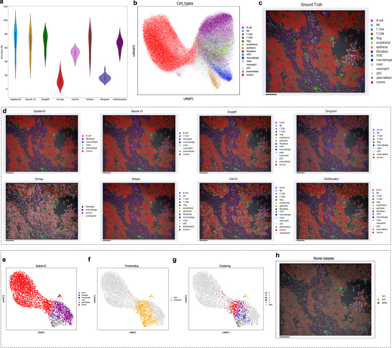
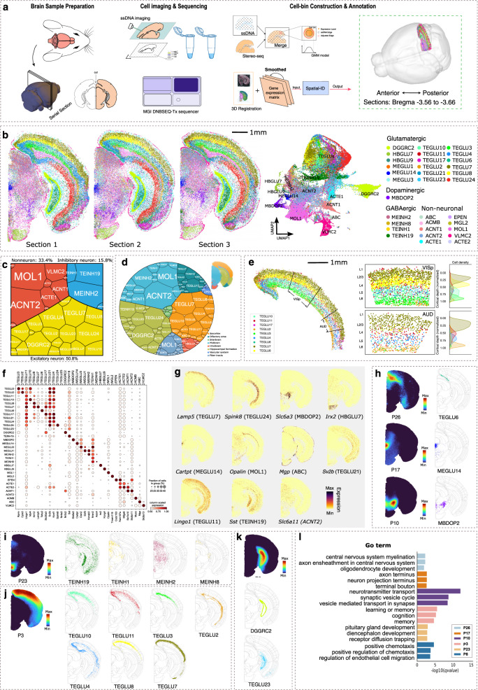
Spatially resolved transcriptomics provides the opportunity to investigate the gene expression profiles and the spatial context of cells in naive state, but at low transcript detection sensitivity or with limited gene throughput. Comprehensive annotating of cell types in spatially resolved transcriptomics to understand biological processes at the single cell level remains challenging. Here we propose Spatial-ID, a supervision-based cell typing method, that combines the existing knowledge of reference single-cell RNA-seq data and the spatial information of spatially resolved transcriptomics data. We present a series of benchmarking analyses on publicly available spatially resolved transcriptomics datasets, that demonstrate the superiority of Spatial-ID compared with state-of-the-art methods. Besides, we apply Spatial-ID on a self-collected mouse brain hemisphere dataset measured by Stereo-seq, that shows the scalability of Spatial-ID to three-dimensional large field tissues with subcellular spatial resolution.

Fig. 1. Overview of Spatial-ID.

Stage 1 involves knowledge transfer from reference datasets. Stage 2 involves feature embedding of gene expression and spatial information, and employs self-supervised strategy to train a classifier (CLS) using the generated pseudo-labels in stage 1. Stage 3 uses the optimal model derived from Stage 2 to perform cell type annotation. a Reference scRNA-seq datasets are employed to pretrain deep neural network (DNN) models. b Based on the cell type probabilities distributions $D$ produced by pretrained DNN, pseudo-labels $L$ are generated by adjusting the temperature parameter $T$. c A deep autoencoder is used to learn encoded gene representation $X$ through reducing the dimension of the gene expression matrix $I$. The gene expression matrix $I^{\prime }$ reconstructed by decoder is used to optimize the autoencoder by minimizing with the input gene expression matrix $I$. d A spatial neighbor graph is constructed to represent the spatial relationships between neighboring cells, where the relationship weight of each pair of cells is negatively associated with Euclidean distance. Therefore, the spatial neighbor graph is represented as an adjacency matrix $A$. e A variational graph autoencoder (VGAE, a kind of GCN) is used to embed the encoded gene representations $X$ from autoencoder and the adjacency matrix $A$, and then generate the spatial embedding $S$ as output. The reconstructed adjacency matrix $A^{\prime }$ is used to optimize the VGAE by minimizing with the input adjacency matrix $A$.

Fig. 2. Application to mouse primary motor cortex dataset measured by MERFISH.

a The MOP region annotations in the Allen CCF v3 (http://atlas.brain-map.org/). b The ground truth cell types using UMAP embedding. c The Spatial-ID prediction using UMAP embedding. d Spatial organization of the ground truth cell types in a coronal slice (slice153). Bar scale 400 μm. e Spatial organization of the Spatial-ID prediction in d. Bar scale 400 μm. f The comparison of cell type annotation accuracy; n = 12 independent samples; center line, median; box limits, upper and lower quartiles; whiskers, 1.5× interquartile range. Notably, the mean accuracy of Cell-ID is 17.08%, that is far below those shown and is therefore not shown. g The confusion matrix of Spatial-ID prediction. The vertical axis and the horizonal axis list the ground truth cell types and the prediction of Spatial-ID, respectively. h The ground truth of L5 ET, L5/6 NP, L6 CT, and L6b neurons, and the prediction of Spatial-ID and the control methods. Bar scale 400 μm. i The neighborhood complexity of a given cell is defined as the number of different cell types presented within a neighborhood of 100 μm in radius. The neighborhood purity of a given cell is defined as the fraction of the most abundant cell type to all cells in the neighborhood of 100 μm in radius. j Simulations of different gene dropout rates. From left to right, the comparison of cell type annotation accuracy at different gene dropout rates, spatial organization of the Spatial-ID prediction at the dropout rate of 0.5, the comparison of cell type annotation accuracy at the dropout rate of 0.5 (n = 12 independent samples; Center line, median; box limits, upper and lower quartiles; whiskers, 1.5× interquartile range), the confusion matrix of Spatial-ID prediction at the dropout rate of 0.5. Bar scale 400 μm. k New cell type discovery. From left to right, ground truth of L4/5 IT and L6 IT Car3 neurons, a pipeline of new cell type discovery, unassigned cells after thresholding, clusters derived from clustering for unassigned cells, and the finally found new cell types (i.e., L4/5 IT and L6 IT Car3). Bar scale 400um.

Fig. 3. Application to mouse hypothalamic preoptic region dataset measured by MERFISH.

a The mouse hypothalamic preoptic region annotations in the Allen CCF v3 (http://atlas.brain-map.org/). b Visualization of the ground truth cell types using UMAP embedding. c Visualization of the Spatial-ID predictions using UMAP embedding. d 3D spatial organization of the ground truth cell types of a sample with naive behavior, and the predictions of Spatial-ID and the control methods. Scale unit (µm). e The comparison of cell type annotation accuracy; n = 3 independent samples; Center line, median; box limits, upper and lower quartiles; whiskers, 1.5× interquartile range. f The confusion matrixes show the fraction of cells from any ground truth cell type predicted by Spatial-ID and control methods. The vertical axis lists the ground truth cell types, and the horizonal axis lists the predicted cell types. Mature OD: Mature oligodendrocyte; Immature OD: Immature oligodendrocyte.

Fig. 4. Application to mouse spermatogenesis dataset measured by Slide-seq.

a Visualization of the ground truth cell types using UMAP embedding. ES elongating spermatid, RS round spermatid, SPC spermatocyte, SPG spermatogonium. b Visualization of the Spatial-ID predictions using UMAP embedding. c The comparison of cell type annotation accuracy; n = 6 independent samples; Center line, median; box limits, upper and lower quartiles; whiskers, 1.5× interquartile range. d Spatial organization of the ground truth cell types of a wild-type sample, and the predictions of Spatial-ID and the control methods. Bar scale 400 µm. e Spatial organization of the ground truth cell types of an ob/ob sample, and the predictions of Spatial-ID and the control methods. Bar scale 400 µm. f The average time cost per sample of Spatial-ID and control methods in this mouse spermatogenesis dataset. The comprehensive results for all SRT datasets in this study can be found in Supplementary Table 3. g The running efficiency analysis. The left one shows the scheme of field view sampling. The right one shows that the runtime of Spatial-ID increases linearly as the number of cells increases. The regression plots of runtimes are presented as mean values with 95% confidence intervals.

Fig. 5. Application to human NSCLC dataset.

a The comparison of cell type annotation accuracy; n = 20 independent samples; Center line, median; box limits, upper and lower quartiles; whiskers, 1.5× interquartile range. Notably, the mean accuracy of SciBet is 0.98%, that is far below those shown and is therefore not shown. b Visualization of the ground truth cell types using UMAP embedding. c Spatial organization of the ground truth cell types of a sample. Field size is about 0.7 mm × 0.9 mm. Bar scale 100 µm. d Spatial organization of the predictions of Spatial-ID and the control methods. Bar scale 100 µm. e Visualization of the predictions of Spatial-ID for this sample using UMAP embedding. f Visualization of the unassigned cells of this sample using UMAP embedding. g Visualization of the clusters of the unassigned cells using UMAP embedding. h Spatial organization of the finally found new cell types. nc1: new class type 1; nc2: new class type 2. Bar scale 100 µm.

Fig. 6. Application to large field mouse brain hemisphere dataset measured by Stereo-seq.

a The workflow of data acquisition, data processing, and cell type annotation. b Cell type annotation of Spatial-ID for the 3 adjacent sections (Bregma −3.56 to −3.66 mm), and UMAP visualization. c A Voronoi treemap shows the composition of excitatory neurons, inhibitory neurons, and non-neuronal cells among the 3 sections. Every tile denotes one cell type and its size represents cell number. d A Voronoi diagram shows cell type organization among distinct brain regions of the 3 sections. Every tile is colored by its populated ABA functional region and its size represents cell number. e Spatial organization of the cortical pyramidal neurons, i.e., TEGLU2, TEGLU3, TEGLU4, TEGLU6, TEGLU7, TEGLU8, TEGLU10, TEGL11, and TEGLU17 in the Section 3. Cells in the VISp and AUD region are individually presented in the middle panel. The right panel shows the kernel density estimate plots for the corresponding cell types along the normalized cortical depth. f The expression dot plots show the gene expression specificity of typical marker genes for identified cell types. Dot size represents the proportion of expressing cells and color indicates average expression level in each identified cell type. g Spatial distributions of selected marker genes show the number of transcripts captured by Stereo-seq. h The spatial gene patterns consist of type-specific genes (Section 3, visualized with pattern scores). The right panel shows the corresponding identified cell types together with the ABA spatial anatomical functional regions. i–k The spatial gene patterns consist of region-specific genes from diverse identified cell types (Section 3). The corresponding identified cell types are illustrated on the right. l Top three highly enriched GO terms for each spatial gene pattern in (h–k).

References

1. Kolodziejczyk AA, et al. The technology and biology of single-cell RNA sequencing. Mol. Cell. 2015;58:610–620. doi: 10.1016/j.molcel.2015.04.005. - DOI - PubMed
1. Svensson V, Vento-Tormo R, Teichmann SA. Exponential scaling of single-cell RNA-seq in the past decade. Nat. Protoc. 2018;13:599–604. doi: 10.1038/nprot.2017.149. - DOI - PubMed
1. Kharchenko PV. The triumphs and limitations of computational methods for scRNA-seq. Nat. Methods. 2021;18:723–732. doi: 10.1038/s41592-021-01171-x. - DOI - PubMed
1. Marx V. Method of the Year: spatially resolved transcriptomics. Nat. Methods. 2021;18:9–14. doi: 10.1038/s41592-020-01033-y. - DOI - PubMed
1. Lewis SM, et al. Spatial omics and multiplexed imaging to explore cancer biology. Nat. Methods. 2021;18:997–1012. doi: 10.1038/s41592-021-01203-6. - DOI - PubMed