Sensor-to-Image Based Neural Networks: A Reliable Reconstruction Method for Diffuse Optical Imaging of High-Scattering Media

Abstract

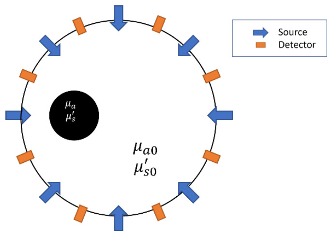
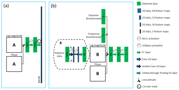
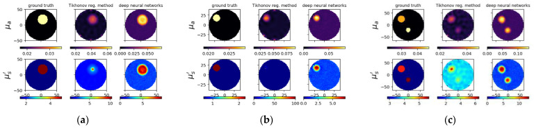
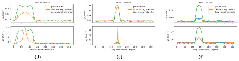
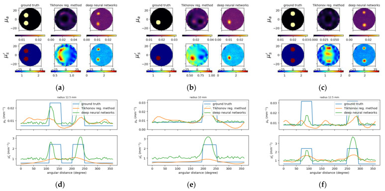
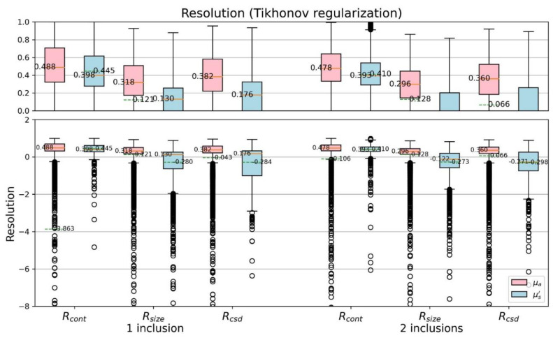
Imaging tasks today are being increasingly shifted toward deep learning-based solutions. Biomedical imaging problems are no exception toward this tendency. It is appealing to consider deep learning as an alternative to such a complex imaging task. Although research of deep learning-based solutions continues to thrive, challenges still remain that limits the availability of these solutions in clinical practice. Diffuse optical tomography is a particularly challenging field since the problem is both ill-posed and ill-conditioned. To get a reconstructed image, various regularization-based models and procedures have been developed in the last three decades. In this study, a sensor-to-image based neural network for diffuse optical imaging has been developed as an alternative to the existing Tikhonov regularization (TR) method. It also provides a different structure compared to previous neural network approaches. We focus on realizing a complete image reconstruction function approximation (from sensor to image) by combining multiple deep learning architectures known in imaging fields that gives more capability to learn than the fully connected neural networks (FCNN) and/or convolutional neural networks (CNN) architectures. We use the idea of transformation from sensor- to image-domain similarly with AUTOMAP, and use the concept of an encoder, which is to learn a compressed representation of the inputs. Further, a U-net with skip connections to extract features and obtain the contrast image, is proposed and implemented. We designed a branching-like structure of the network that fully supports the ring-scanning measurement system, which means it can deal with various types of experimental data. The output images are obtained by multiplying the contrast images with the background coefficients. Our network is capable of producing attainable performance in both simulation and experiment cases, and is proven to be reliable to reconstruct non-synthesized data. Its apparent superior performance was compared with the results of the TR method and FCNN models. The proposed and implemented model is feasible to localize the inclusions with various conditions. The strategy created in this paper can be a promising alternative solution for clinical breast tumor imaging applications.

Keywords: Tikhonov regularization (TR); convolutional neural networks; deep modeling; diffuse optical imaging; image reconstruction; inverse problem; residual net; skip connection.

Figure 1

Illustration of optical information measurement for DOT imaging.

Figure 2

Flowcharts of image reconstruction methods. (a) Iterative method and (b) deep neural network.

Figure 3

Some examples of training phantom designs with varied parameters, where D, r, r_oc and θ denote phantom diameter, inclusion radius, off-center distance of inclusion(s) and orientation of inclusion(s), respectively.

Figure 4

Block diagram of the proposed model, where $\mathsf{\Phi }$, $\mathrm{f}$ and $\mathrm{d}$ denote input radiance, FD frequency and phantom diameter, respectively.

Figure 5

Proposed deep learning model including (a) domain-transform and (b) background predictor.

Figure 6

Network architecture of the block A.

Figure 7

Measurement calibration: (a) calibration phantom (top and lateral views); (b) 3D scanning system with the calibration phantom; (c) flowchart of calibration procedure; and (d) standard deviations of measured data in mV for 30 detections [32].

Figure 8

Loss during training and validation phases along with iteration epochs.

Figure 9

Reconstructed images for simulated cases A1675, A4144 and A6392 from left to right, respectively. (a–c) Designated and computed optical-property images, (upper) μ_a and (lower) ${\mu }_s^{\prime }$ image; in (a–c), (left) ground truth, and reconstructed images using (middle) TR and (right) deep neural networks. (d–f) Circular cross-section profile of (upper) μ_a and (lower) ${\mu }_s^{\prime }$ distribution that intersects with an (outer) inclusion.

Figure 9

Reconstructed images for simulated cases A1675, A4144 and A6392 from left to right, respectively. (a–c) Designated and computed optical-property images, (upper) μ_a and (lower) ${\mu }_s^{\prime }$ image; in (a–c), (left) ground truth, and reconstructed images using (middle) TR and (right) deep neural networks. (d–f) Circular cross-section profile of (upper) μ_a and (lower) ${\mu }_s^{\prime }$ distribution that intersects with an (outer) inclusion.

Figure 10

Reconstructed images for experimental case B2, B3 and B7 from left to right, respectively. (a–c) Designated and computed optical-property images, (upper) μ_a and (lower) ${\mu }_s^{\prime }$ image; in (a–c), (left) ground truth, and reconstructed images using (middle) TR and (right) deep neural networks. (d–f) Circular cross-section profile of (upper) μ_a and (lower) ${\mu }_s^{\prime }$ distribution that intersects with the center of inclusions.

Figure 11

The same caption as in Figure 9 except the reconstructed images (a–c) on the (right) using FCNN and one of circular cross-section profiles using FCNN (d–f).

Figure 11

The same caption as in Figure 9 except the reconstructed images (a–c) on the (right) using FCNN and one of circular cross-section profiles using FCNN (d–f).

Figure 12

The same caption as in Figure 10 except the reconstructed images (a–c) on the (right) using FCNN and one of circular cross-section profiles using FCNN (d–f).

Figure 13

Scatter plots of the CSD resolution for one-inclusion samples. (a,b) show the resolutions for absorption (μ_a) while (c,d) for reduced scattering (${\mu }_s^{\prime }$). Besides, on the left (a,c) from Tikhonov regularization while on the right (b,d) from proposed model.

Figure 14

Boxplots of CSD resolution (TR).

Figure 15

Boxplots of CSD resolution (proposed model).

Figure 16

Boxplots of MSE for $\frac{\mu }{{\mu }_{base}}$ (TR).

Figure 17

Boxplots of MSE for $\frac{\mu }{{\mu }_{base}}$ (proposed model).

References

1. Krizhevsky A., Sutskever I., Hinton G.E. ImageNet Classification with Deep Convolutional Neural Networks. Commun. ACM. 2017;60:84–90. doi: 10.1145/3065386. - DOI
1. Ronneberger O., Fischer P., Brox T. Lecture Notes in Computer Science (Including Subseries Lecture Notes in Artificial Intelligence and Lecture Notes in Bioinformatics) Volume 9351. Springer International Publishing; Cham, Switzerland: 2015. U-Net: Convolutional Networks for Biomedical Image Segmentation; pp. 234–241. - DOI
1. Pelt D.M., Batenburg K.J. Fast Tomographic Reconstruction from Limited Data Using Artificial Neural Networks. IEEE Trans. Image Process. 2013;22:5238–5251. doi: 10.1109/TIP.2013.2283142. - DOI - PubMed
1. Wang S., Su Z., Ying L., Peng X., Zhu S., Liang F., Feng D., Liang D. Accelerating Magnetic Resonance Imaging via Deep Learning. Proc.-Int. Symp. Biomed. Imaging. 2016;2016:514–517. doi: 10.1109/ISBI.2016.7493320. - DOI - PMC - PubMed
1. Zhu B., Liu J.Z., Cauley S.F., Rosen B.R., Rosen M.S. Image Reconstruction by Domain-Transform Manifold Learning. Nature. 2018;555:487–492. doi: 10.1038/nature25988. - DOI - PubMed
MeSH terms
LinkOut - more resources