The InSight HP3 Penetrator (Mole) on Mars: Soil Properties Derived from the Penetration Attempts and Related Activities

Abstract

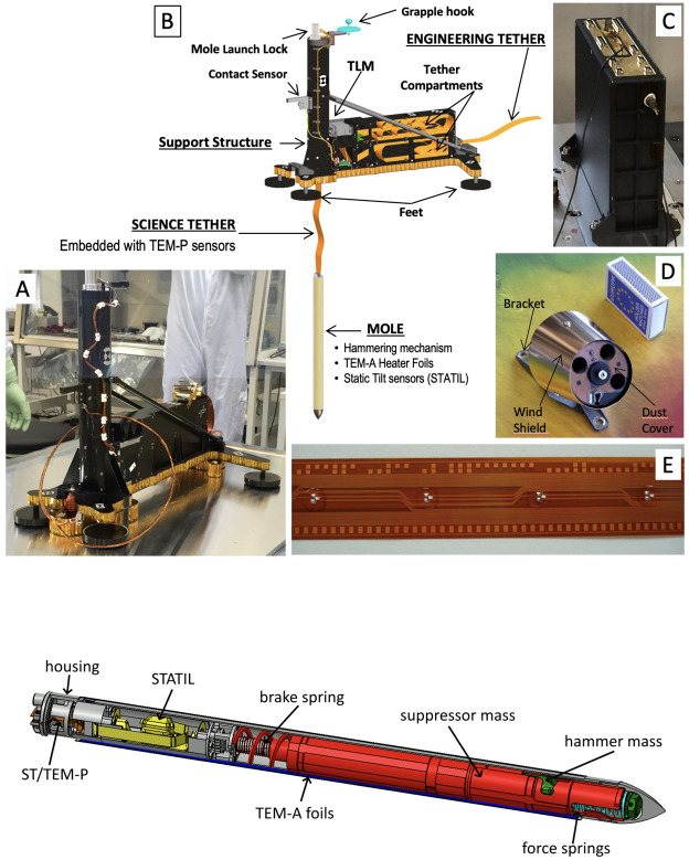
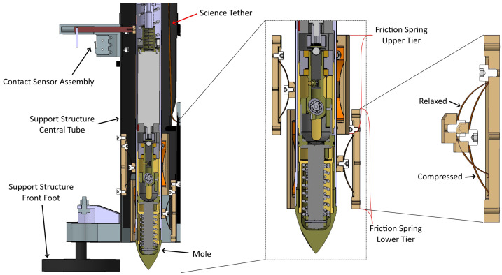
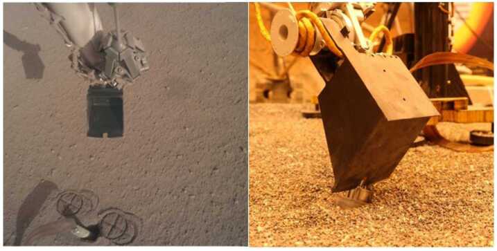
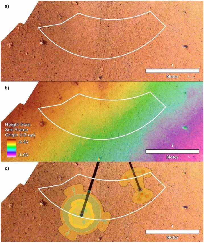
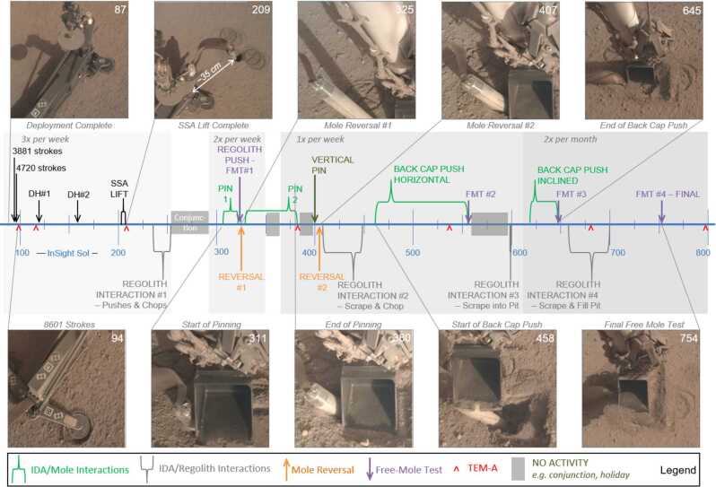
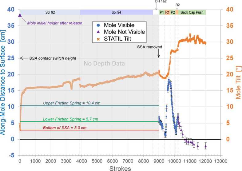
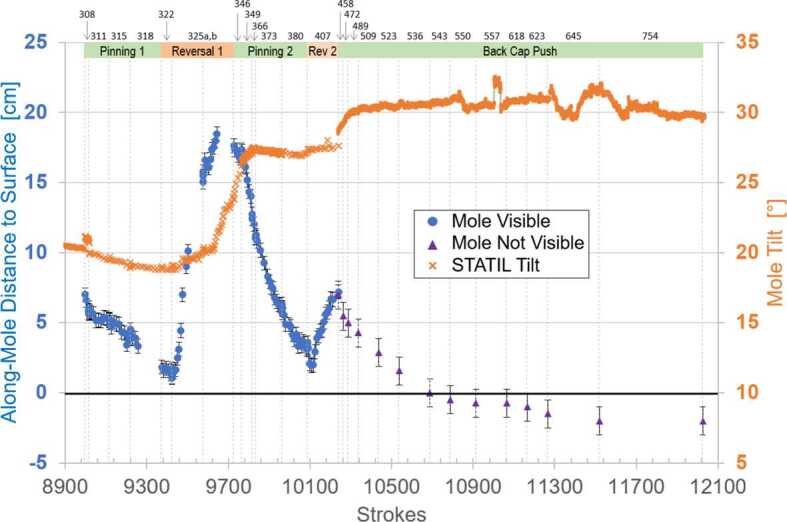
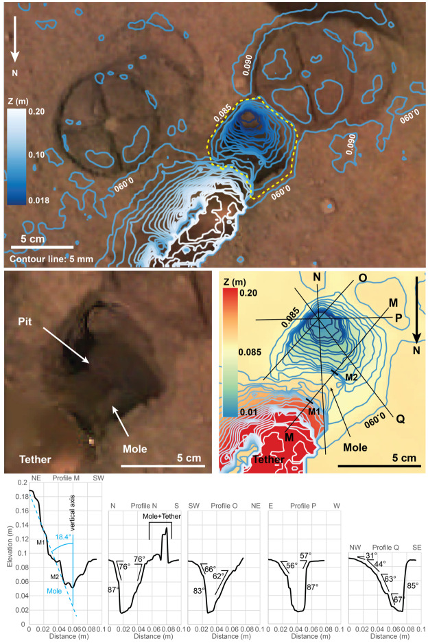
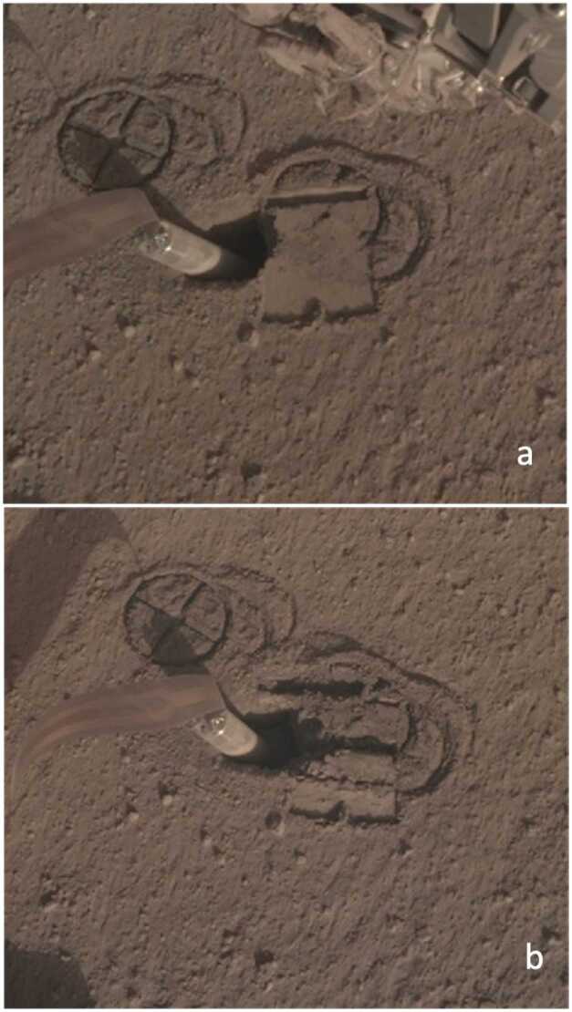
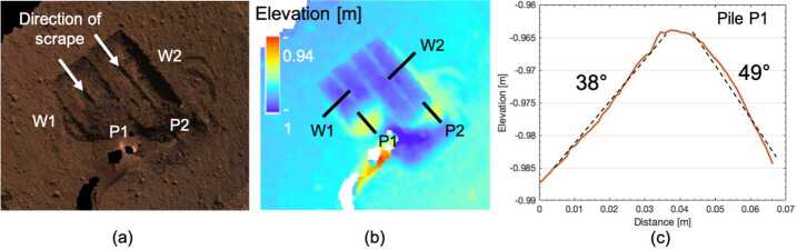
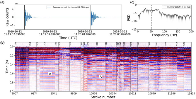
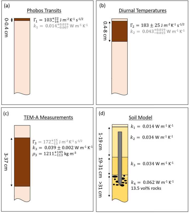
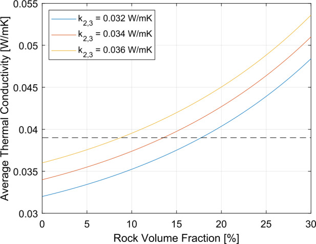
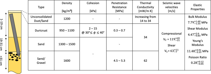
The NASA InSight Lander on Mars includes the Heat Flow and Physical Properties Package HP³ to measure the surface heat flow of the planet. The package uses temperature sensors that would have been brought to the target depth of 3-5 m by a small penetrator, nicknamed the mole. The mole requiring friction on its hull to balance remaining recoil from its hammer mechanism did not penetrate to the targeted depth. Instead, by precessing about a point midway along its hull, it carved a 7 cm deep and 5-6 cm wide pit and reached a depth of initially 31 cm. The root cause of the failure - as was determined through an extensive, almost two years long campaign - was a lack of friction in an unexpectedly thick cohesive duricrust. During the campaign - described in detail in this paper - the mole penetrated further aided by friction applied using the scoop at the end of the robotic Instrument Deployment Arm and by direct support by the latter. The mole tip finally reached a depth of about 37 cm, bringing the mole back-end 1-2 cm below the surface. It reversed its downward motion twice during attempts to provide friction through pressure on the regolith instead of directly with the scoop to the mole hull. The penetration record of the mole was used to infer mechanical soil parameters such as the penetration resistance of the duricrust of 0.3-0.7 MPa and a penetration resistance of a deeper layer ( $>30\text{cm}$ depth) of $4.9\pm 0.4\text{MPa}$ . Using the mole's thermal sensors, thermal conductivity and diffusivity were measured. Applying cone penetration theory, the resistance of the duricrust was used to estimate a cohesion of the latter of 2-15 kPa depending on the internal friction angle of the duricrust. Pushing the scoop with its blade into the surface and chopping off a piece of duricrust provided another estimate of the cohesion of 5.8 kPa. The hammerings of the mole were recorded by the seismometer SEIS and the signals were used to derive P-wave and S-wave velocities representative of the topmost tens of cm of the regolith. Together with the density provided by a thermal conductivity and diffusivity measurement using the mole's thermal sensors, the elastic moduli were calculated from the seismic velocities. Using empirical correlations from terrestrial soil studies between the shear modulus and cohesion, the previous cohesion estimates were found to be consistent with the elastic moduli. The combined data were used to derive a model of the regolith that has an about 20 cm thick duricrust underneath a 1 cm thick unconsolidated layer of sand mixed with dust and above another 10 cm of unconsolidated sand. Underneath the latter, a layer more resistant to penetration and possibly containing debris from a small impact crater is inferred. The thermal conductivity increases from 14 mW/m K to 34 mW/m K through the 1 cm sand/dust layer, keeps the latter value in the duricrust and the sand layer underneath and then increases to 64 mW/m K in the sand/gravel layer below.

Supplementary information: The online version contains supplementary material available at 10.1007/s11214-022-00941-z.

Keywords: Homestead Hollow near surface structure; Martian soil mechanical and thermal properties; Record of operating a penetrator on Mars.

Fig. 1

Elements of the Heat Flow and Physical Properties Package (HP³). (A) Flight model Support System Assembly (SSA). (B) Annotated cutaway of the SSA showing Mole and Engineering Tether partly deployed. (C) Back End Electronics within the InSight lander, (D) Deck-mounted HP³ Radiometer (matchbox for scale). (E) Science Tether showing embedded TEM-P sensors, relative depth markings (bottom) and Gray binary code absolute depth markings (top). A prototype with closely spaced sensors is shown here for illustration; the actual flight Science Tether has greater (and irregular) spacing between sensors. The bottom panel shows an annotated cutaway of the HP³ mole (from Spohn et al. 2022) with the tiltmeter STATIL (yellow), the Science Tether ST/TEM-P attachment (orange), the TEM-A foils (purple), the suppressor mass including the brake spring of the hammering mechanism (red), the hammer mass (green), the force springs (light blue) and the housing (grey)

Fig. 2

This partial cross-section of the forward-front portion of the Support Structure shows the mole in its position prior to penetration. The contact sensor assembly position (top left) allows it to indicate when the mole has moved 14.8 cm out of the tube. The outlines at the center and right show the positions of the upper and lower friction spring tiers, and also the shape of the springs in their relaxed and compressed states. A portion of the Science Tether service loop can also be seen extending up from the TLM towards the back cap of the mole (not pictured)

Fig. 3

The Instrument Deployment System

Fig. 4

The IDA scoop. In the left image, the scoop is shown above the HP³ mole in this IDC image. The front blade is visible. The grapple is seen stowed to the side of the IDA forearm. In the right image, the scoop in the Earth-based testbed is shown in an “inclined push” configuration on the testbed mole back cap. The dull blade on the outside back of the scoop is visible

Fig. 5

Image mosaic, DEM, and instrument placements selected by the ISSWG and project. (a) The first IDC image mosaic created of the workspace at 1 mm/pixel with the deployment area outlined in white. (b) High-resolution DEM produced from the second mosaic of the workspace at 1 mm per elevation posting and the deployment area outlined in white. Note that the deployment area has a total relief measured in centimeters. (c) Locations selected for the instruments with black lines to the instrument grapple points. SEIS and WTS are to the left and HP³ is to the right. North is up for all

Fig. 6

This linear timeline shows key periods (braces) and events (arrows and carets) of the mole penetration anomaly from the end of SSA deployment (Sol 87) to the final Free-Mole Test (Sol 764). Callout figures with sol numbers in the upper right show selected zoomed views from the IDC. Shaded background regions indicate changes in operational cadence

Fig. 7

This plot shows (left axis, circles and triangles) the distance along-mole from the mole back cap to the original regolith surface (zero datum), and the tilt of the mole with respect to local gravity (right axis, x’s) as measured by STATIL; both axes are referenced to the total number of hammer strokes accumulated since sol 92. Blue circles indicate along-mole distance to datum as determined from IDC images of glint features on the mole back cap. Filled purple triangles indicate along-mole distance determined through various indirect means (e.g., SSA contact switch or IDA scoop/regolith relative position)

Fig. 8

This plot zooms in on data shown in Fig. 7 beginning on sol 308 when the first pinned-mole hammering test was executed. Symbol colors and meanings are the same as in Fig. 7. Note the different scales for the left-hand axis (back-cap distance to surface) and right-hand axis (mole tilt from STATIL). Individual sols where hammering occurred are indicated along the top border; vertical dashed lines show the boundaries of each sol’s planned hammer strokes. The major periods of successful mole penetration (Pinning 1, Pinning 2, and Back Cap Push) are indicated by green horizontal bars along the top, while major periods of mole reversal (Reversal 1 and Reversal 2) are in orange

Fig. 9

Digital elevation model of the pit based on a $4\times 4\times 1$ IDC imaging data set taken on sol 230 after SSA replacement and using virtual control point methods. The top frame shows 5 mm depth interval contour lines superimposed on the orthorectified image mosaic. The rim of the pit is marked by a yellow dashed line. In addition to the pit, the imprints of the SSA feet in the fine-grained surface layer are clearly seen as well as the tether connected to the back-end of the mole. Below the top frame, from left to right, a close up orthorectified image of the pit is shown and a colour-digital elevation model (DEM) of the pit in which the reference elevation plane is 2 cm below the deepest point of the pit. Labelled black lines correspond to the location of topographic profiles M–Q shown in the panels in the bottom row. Profile M extends all along the mole between points M1 and M2 and up the tether. The average slope between M1 and M2 is ${18.4}^{\circ }$ which compares well with the tilt angle of the mole measured by STATIL of $20\pm 1^{\circ }$. Selected measured topographic slopes are given

Fig. 10

Image of the hole created by the HP³ mole showing the almost vertical southerly wall of the pit and resistant layers in it. These layers have steep edges and overhangs indicating cohesion in the soil. Small rocks appear cemented in a fine-grained matrix, similar to the pits beneath the lander. Mole is in the foreground angled $\sim {15}^{\circ }$ towards the right

Fig. 11

Image of mole hole and surface after interactions with the HP³ SSA feet and scoop. Circular cross patterns are imprints of the HP³ SSA feet in the soil. Smooth, reflective rectangular surface is where the flat base of the scoop (7.1 cm wide) was pressed against the soil, causing a 5–10 mm indentation. Horizontal troughs near the top and bottom of the scoop imprint are where the front and back blades of the scoop (Fig. 4) penetrated into the soil

Fig. 12

Top: Reading of the x-y sensors of STATIL during the first 325 hammer strokes on Sol 92 in degrees. The recordings are ambiguous with respect to rotation of the mole and x-y motion of the tip. The recordings are consistent, however, with a south and west movement of the tip and followed by a northward rotation of the mole as suggested by the position and the attitude of the mole and the twisted orientation of the tether in images taken at Sol 230. Bottom: Reconstructed path of the back-cap from the footprints of the feet using the known dimensions of the support structure. While STATIL data indicate a movement of the tip southward and then westward, the back-cap moved northeastward and then eastward

Fig. 13

Statil recording of the first 500 strokes on sol 92. Marked are the mole passage of the contact switch as sensed by STATIL and the stroke when the mole tip suddenly changed direction from mostly southward to mostly northward (compare Fig. 12). Note that because of the ambiguity in the STATIL data the inferred change in direction of tip movement may also be a sudden change in sense of rotation. Also note the wavy character of the increase in tilt angle after stroke 200

Fig. 14

Illustration of the support structure lift and rotation about an axis through its back feet as suggested by the interpretation of the STATIL data recorded on sol 92 and discussed in Sect. 6.2.1

Fig. 15

Data used to estimate the penetration resistances of the layers the mole penetrated or attempted to penetrate. Plotted are the “Along-Mole Distances to the Surface” in centimeters and the “Mole Tilt” in degrees as functions of the cumulative number of strokes at the sols indicated. The top left panel shows the estimate of the along-mole distance after 77 strokes on sol 92 at the time of the back-cap passing the contact switch in the SSA (compare text) and the evolution of the tilt from $4^{\circ }$ to ${11}^{\circ }$. The top-right panel shows the progress of the mole by 5 cm between sols 308 and 322 and the change of the tilt by about $1^{\circ }$. The bottom left panel gives the data for the re-penetration after mole extraction during sols 346–380. The bottom right panel shows the penetration by about 6 cm during sols 458–536 accompanied by an initial increase in tilt by about $2^{\circ }$ keeping mostly steady thereafter

Fig. 16

Configuration of the scoop during regolith push. The left panel shows the scoop pressed onto the surface next to the mole for the intended regolith push on Sol 322. The right panel shows the mole pit, the backed-out mole and the scoop indentation after lifting the scoop on Sol 333

Fig. 17

Images of IDA scoop interactions with the surface material near the HP³ mole pit. (a) After a flat push on Sol 240. (b) After a tip push on Sol 250

Fig. 18

Digital elevation model of the pit based on the stereo pair taken on sol 673 after IDA scraping. (a) Orthoimage showing the piles P1 and P2 and walls W1 and W2 left after the scoop scraped the regolith. (b) Digital elevation model (c) Elevation profile for pile P1

Fig. 19

Seismic data collected during HP³ mole hammering. The SEIS SP data were recorded with an adapted acquisition procedure that allowed reconstructing the broadband waveforms. (a) Waveforms of two subsequent mole strokes separated by around 3.7 s recorded during the diagnostic hammering on sol 158. Vertical black lines mark the hammering time. (b) All broadband east-component SP data recorded for hammering sessions between sol 158 and 632. Vertical bars show the beginnings of the sessions marked with the corresponding sol. Time $t=0$ s corresponds to the mole hammering time. The seismic signal show clear first arriving energy being interpreted as the P-wave arrival. The mole hammer strokes also excite the 25-Hz resonance denoted with A, which is assumed to originate from vibrations of the SEIS housing and/or leveling system. (c) Power spectral density computed for all data recorded during the hammering on sol 311. Note how the frequency bandwidth of the hammer signal exceeds the Nyquist frequency of 50 Hz of the nominal SEIS acquisition (marked by the dashed line) highlighting the value of the reconstruction method by Sollberger et al. (2021)

Fig. 20

(a)–(c) Summary of regolith physical properties derived from HP³ RAD and active heating experiments using TEM-A. The sensing depths of the different methods are indicated. Quantities that are immediately calculated from the data such as thermal inertia in panels a and b and thermal conductivity and density in panel c are given in black. Values inferred from the data are given in gray. To convert thermal conductivity to thermal inertia, a soil heat capacity of $630\text{J}{\text{kg}}^{-1}{\text{K}}^{-1}$ has been assumed (Morgan et al. 2018). (d) Soil thermal model compatible with all observations assuming four regolith layers: A top unconsolidated sand/dust layer, a duricrust, an unconsolidated sand layer, as well as a layer including small rocks or gravel. Thermal conductivity of the rocks was assumed to be $3\text{W}{\text{m}}^{-1}{\text{K}}^{-1}$

Fig. 21

Average thermal conductivity in the 3 to 37 cm depth range as a function of the volume fraction of stones in a hypothetical gravel layer located below 31 cm depth (compare Fig. 20). Results are shown for three different thermal conductivities $k_{2,3}$ of the uppermost duricrust and intermediate sand layer, respectively. The average thermal conductivity of the entire soil column as measured using TEM-A is indicated by the horizontal dashed line. For 100 μm diameter particles, $k=0.032$ to $0.036\text{W}{\text{m}}^{-1}{\text{K}}^{-1}$ (Presley and Christensen 1997). Thus the volume fraction of rocks is limited to be smaller than 18%

Fig. 22

Model of the martian soil at the HP³ mole pit. The assumed range of internal friction angle $\varphi$ for the listed cohesion value range is indicated

References

1. Abarca H, Deen R, Hollins G, Zamani P, Maki J, Tinio A, Pariser O, Ayoub F, Toole N, Algermissen S, Soliman T, Lu Y, Golombek M, Calef F, Grimes K, De Cesare C, Sorice C. Image and data processing for InSight lander operations and Science. Space Sci Rev. 2019;215(B9):14,095–14,104. doi: 10.1007/s11214-019-0587-9. - DOI
1. ASTM C1444-00 (2000) Standard test method for measuring the angle of repose of free-flowing mold powders. Standard, ASTM International, West Conshohocken, PA, USA
1. Banaszkiewicz M, Seiferlin K, Spohn T, Kargl G, Koemle N. A new method for the determination of thermal conductivity and thermal diffusivity from line heat source measurements. Rev Sci Instrum. 1997;68:4184–4187. doi: 10.1063/1.1148365. - DOI
1. Banerdt WB, Smrekar SE, Banfield D, Giardini D, Golombek M, Johnson CL, Lognonné P, Spiga A, Spohn T, Perrin C, Stähler SC, Antonangeli D, Asmar S, Beghein C, Bowles N, Bozdag E, Chi P, Christensen U, Clinton J, Collins GS, Daubar I, Dehant V, Drilleau M, Fillingim M, Folkner W, Garcia RF, Garvin J, Grant J, Grott M, Grygorczuk J, Hudson T, Irving JCE, Kargl G, Kawamura T, Kedar S, King S, Knapmeyer-Endrun B, Knapmeyer M, Lemmon M, Lorenz R, Maki JN, Margerin L, McLennan SM, Michaut C, Mimoun D, Mittelholz A, Mocquet A, Morgan P, Mueller NT, Murdoch N, Nagihara S, Newman C, Nimmo F, Panning M, Pike WT, Plesa AC, Rodriguez S, Rodriguez-Manfredi JA, Russell CT, Schmerr N, Siegler M, Stanley S, Stutzmann E, Teanby N, Tromp J, van Driel M, Warner N, Weber R, Wieczorek M. Initial results from the InSight mission on Mars. Nat Geosci. 2020;13:183–189. doi: 10.1038/s41561-020-0544-y. - DOI
1. Banin A, Clark BC, Waenke H. Surface chemistry and mineralogy. In: George M, editor. Mars. Tucson: University of Arizona Press; 1992. pp. 594–625.
LinkOut - more resources