Inferring predator-prey interactions from camera traps: A Bayesian co-abundance modeling approach

Abstract

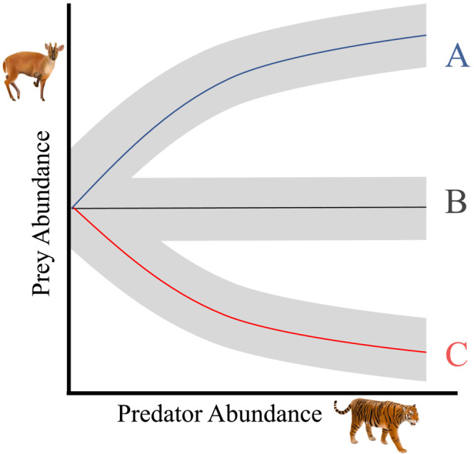
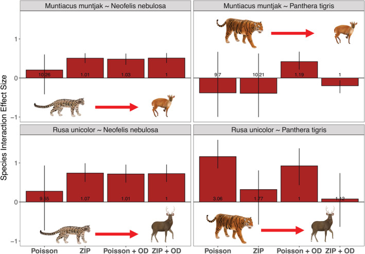
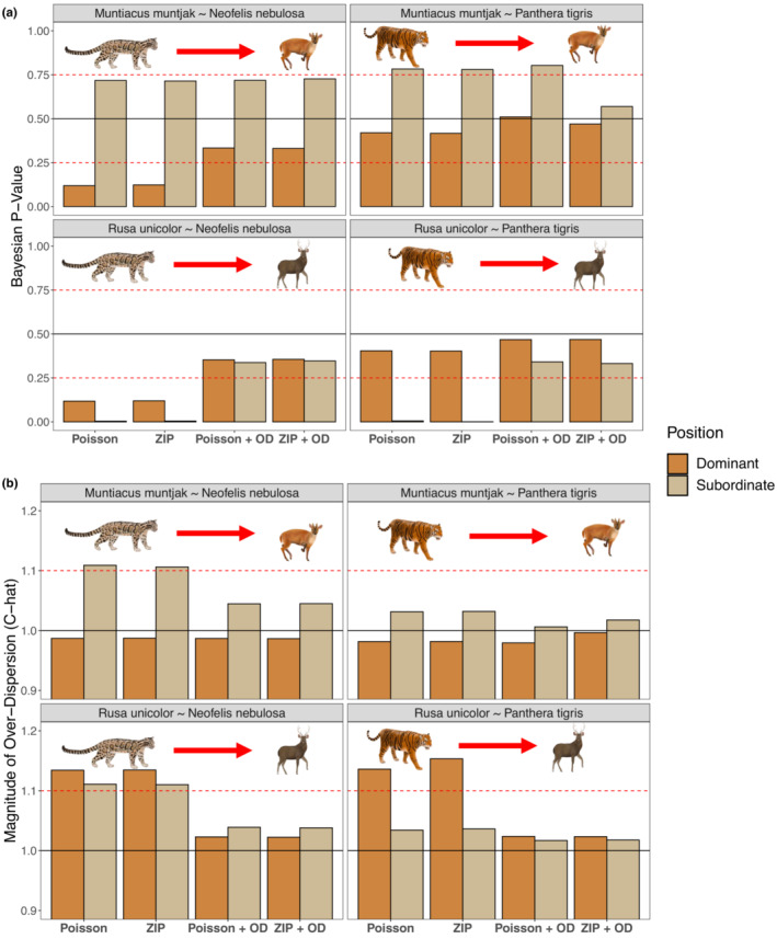
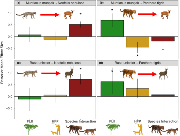
Predator-prey dynamics are a fundamental part of ecology, but directly studying interactions has proven difficult. The proliferation of camera trapping has enabled the collection of large datasets on wildlife, but researchers face hurdles inferring interactions from observational data. Recent advances in hierarchical co-abundance models infer species interactions while accounting for two species' detection probabilities, shared responses to environmental covariates, and propagate uncertainty throughout the entire modeling process. However, current approaches remain unsuitable for interacting species whose natural densities differ by an order of magnitude and have contrasting detection probabilities, such as predator-prey interactions, which introduce zero inflation and overdispersion in count histories. Here, we developed a Bayesian hierarchical N-mixture co-abundance model that is suitable for inferring predator-prey interactions. We accounted for excessive zeros in count histories using an informed zero-inflated Poisson distribution in the abundance formula and accounted for overdispersion in count histories by including a random effect per sampling unit and sampling occasion in the detection probability formula. We demonstrate that models with these modifications outperform alternative approaches, improve model goodness-of-fit, and overcome parameter convergence failures. We highlight its utility using 20 camera trapping datasets from 10 tropical forest landscapes in Southeast Asia and estimate four predator-prey relationships between tigers, clouded leopards, and muntjac and sambar deer. Tigers had a negative effect on muntjac abundance, providing support for top-down regulation, while clouded leopards had a positive effect on muntjac and sambar deer, likely driven by shared responses to unmodelled covariates like hunting. This Bayesian co-abundance modeling approach to quantify predator-prey relationships is widely applicable across species, ecosystems, and sampling approaches and may be useful in forecasting cascading impacts following widespread predator declines. Taken together, this approach facilitates a nuanced and mechanistic understanding of food-web ecology.

Keywords: N‐mixture models; detection probability; hierarchical modeling; overdispersion; species interactions; zero inflation.

FIGURE 1

Hypothetical predator–prey co‐abundance relationships. (a) A positive predator–prey relationship suggests top‐down regulation via predation is not the dominant factor shaping abundances. This may arise where there is strong bottom‐up regulation of both prey and predators or severe disturbances affecting both species. (b) The lack of a predator–prey relationship could arise due to a lack of interactions, such as if predator dietary preferences exclude a specific prey species or each species utilizes different habitats. (c) A negative predator–prey relationship could arise from strong top‐down regulation via predation that regulates prey abundance. Similarly, a negative predator–prey relationship suggests predator extirpation may allow prey to increase, termed “trophic release”.

FIGURE 2

Comparing the effect sizes, 95% Bayesian credibility interval, and parameter convergence (Rhat values) of the species interaction parameter in all four species pairs from our two‐species N‐mixture models. We examined the original two‐species N‐mixture model proposed by Brodie et al. (2018) (Poisson), then examined the addition of the iZIP parameter (ZIP) and ODRE parameter (Poisson + OD) separately, and finally compared our final models that include both the iZIP and ODRE parameters (ZIP + OD). The Y‐axis represents the mean effect sizes of the species interaction parameter, and the error bars represent the 95% Bayesian credibility interval. Finally, the values at the bottom of the bar graphs represent the specific Rhat scores from the species interaction parameter associated with each model.

FIGURE 3

Comparing the goodness‐of‐fit between models by inspecting Bayesian p‐values (a) and the magnitude of overdispersion C‐hat values (b) across four species pairs. We examined the original two‐species N‐mixture model proposed by Brodie et al. (2018) (Poisson), then examined the addition of the iZIP parameter (ZIP) and ODRE parameter (Poisson + OD) separately, and finally compared our final models that include both the iZIP and ODRE parameters (ZIP + OD). (a) Bayesian p‐values are calculated by taking the mean value of the number of times data simulated from the joint posterior distribution was greater than the real data supplied to the model, where Bayesian p‐values between .25 and .75 indicate good fit, a value of 0.5 indicates a perfect fit, and values above or below the dashed red lines (<0.25 or >0.75) indicate a lack of fit. (b) C‐hat values are calculated by dividing the observed data supplied to the model from data simulated from the joint posterior distribution and we visualized the mean value, where C‐hat values greater than 1.1 indicate remaining overdispersion and values close to 1 indicate no remaining overdispersion. A horizontal line is added at 1 to indicate the ideal value for our C‐hat scores, while the red dashed line at 1.1 denotes our cut‐off point for C‐hat values that suggest overdispersion. Both dominant (darker tan color) and subordinate (lighter tan color) species are included in both figures.

FIGURE 4

Parameters describing prey species abundance from the Bayesian co‐abundance models using the informed zero‐inflated Poisson (iZIP) distribution and ODRE. Plots show the posterior mean effect size, and the error bars represent the 95% Bayesian credibility interval (CI), with asterisks (*) denoting relationships where the 95% CI does not include zero. The variables are FLII (green), HFP (yellow), and the species interaction (red), which shows the effect of the dominant (predator) on the subordinate (prey).

FIGURE 5

Predator–prey relationships estimated from the Bayesian co‐abundance models using the iZIP distribution and ODRE. The thick black trend line comes from the posterior distribution of the species interaction parameter, the gray shaded area shows the 95% Bayesian credibility interval (CI), and a solid trend line indicates the 95% CI does not include zero. The points show the estimated species abundances at each sampling unit, colored by landscape. The landscape abbreviations used in the legend are as follows: BBS refers to Bukit Barisan Selatan National Park, Danum Valley refers to Danum Valley Conservation Area, Kerinci refers to Kerinci Seblat National Park, Khao Chong refers to Khao Ban Tat Wildlife Sanctuary, Khao Yai refers to Khao Yai National Park, Lambir refers to Lambir Hills National Park, Leuser refers to Gunung Leuser National Park, Pasoh refers to Pasoh Forest Reserve, Singapore refers to the Central Catchment Nature Reserve and Palau Ubin, and finally Ulu Muda refers to the Greater Ulu Muda Forest Complex.

References

1. Amir, Z. , Moore, J. H. , Negret, P. J. , & Luskin, M. S. (2022). Megafauna extinctions produce idiosyncratic Anthropocene assemblages. Science Advances, 8(42), eabq2307. - PMC - PubMed
1. Atkins, J. L. , Long, R. A. , Pansu, J. , Daskin, J. H. , Potter, A. B. , Stalmans, M. E. , Tarnita, C. E. , & Pringle, R. M. (2019). Cascading impacts of large‐carnivore extirpation in an African ecosystem. Science, 364, 173–177. 10.1126/science.aau3561 - DOI - PubMed
1. Benítez‐López, A. , Santini, L. , Schipper, A. M. , Busana, M. , & Huijbregts, M. A. J. (2019). Intact but empty forests? Patterns of hunting‐induced mammal defaunation in the tropics. PLoS Biology, 17, e3000247. 10.1371/journal.pbio.3000247 - DOI - PMC - PubMed
1. Blanchet, F. G. , Cazelles, K. , Gravel, D. , & Jeffers, E. (2020). Co‐occurrence is not evidence of ecological interactions. Ecology Letters, 23, 1050–1063. 10.1111/ele.13525 - DOI - PubMed
1. Blasco‐Moreno, A. , Pérez‐Casany, M. , Puig, P. , Morante, M. , & Castells, E. (2019). What does a zero mean? Understanding false, random and structural zeros in ecology. Methods in Ecology and Evolution, 10, 949–959. 10.1111/2041-210x.13185 - DOI
LinkOut - more resources