Nano3P-seq: transcriptome-wide analysis of gene expression and tail dynamics using end-capture nanopore cDNA sequencing

Abstract

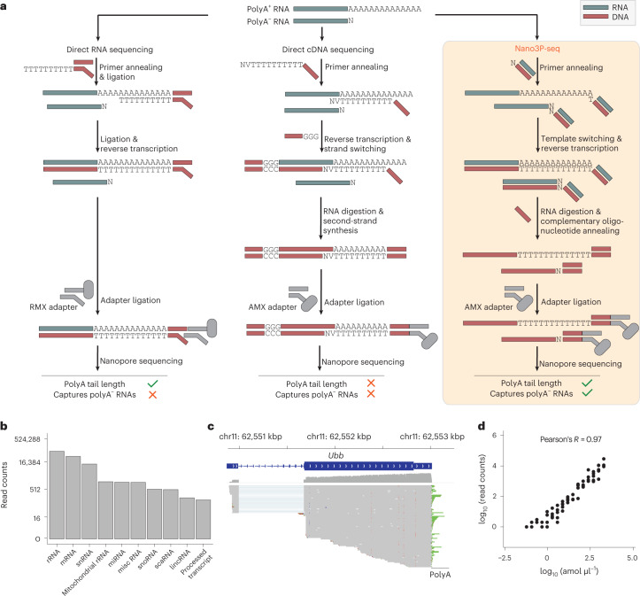
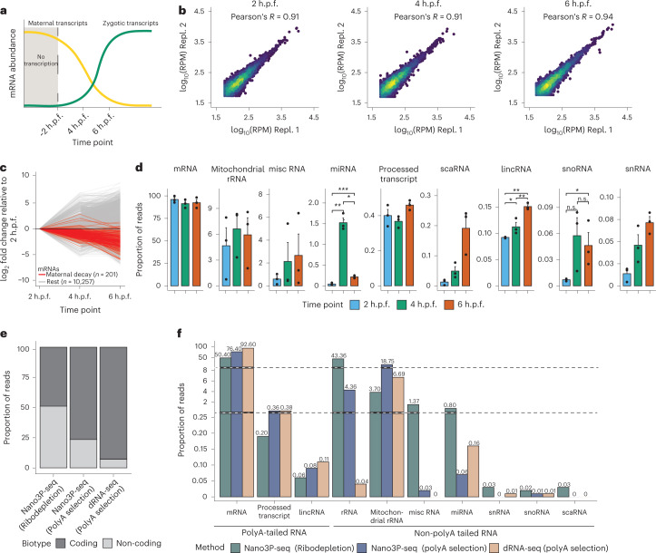
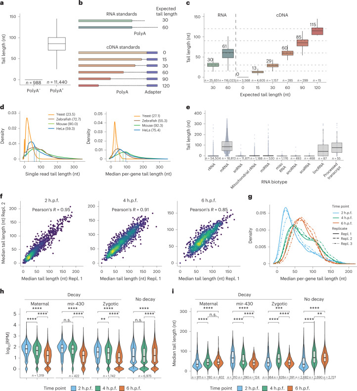
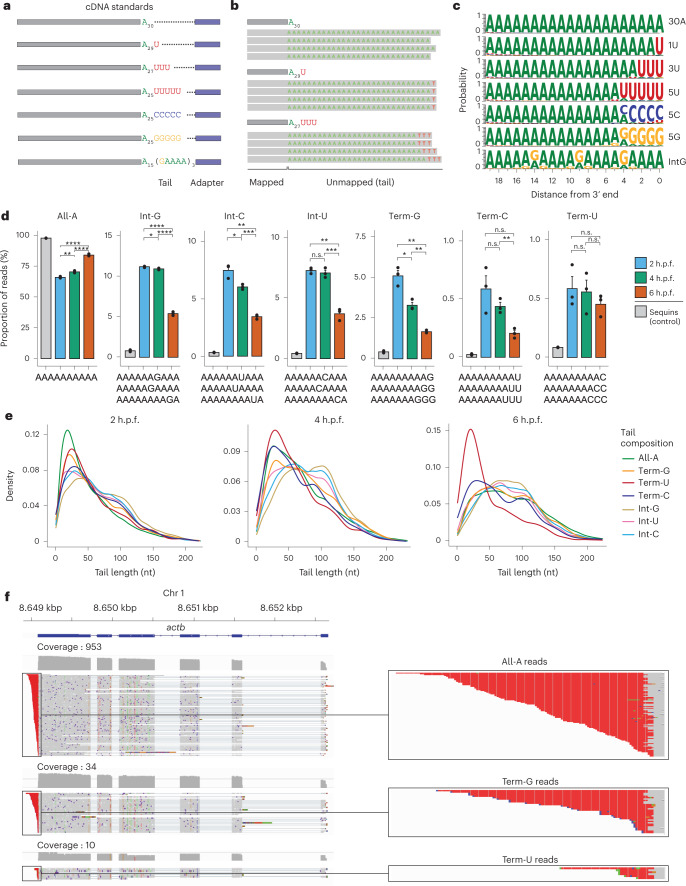
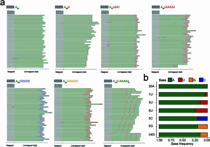
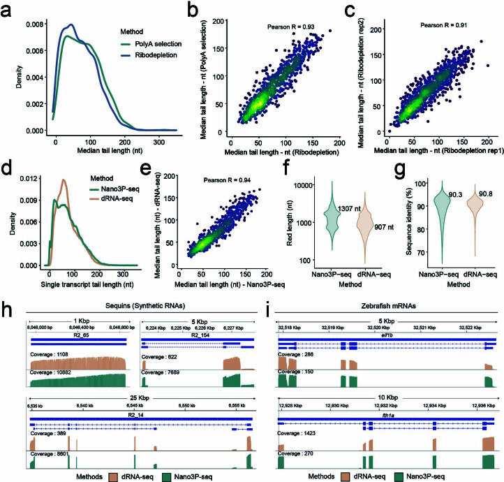
RNA polyadenylation plays a central role in RNA maturation, fate, and stability. In response to developmental cues, polyA tail lengths can vary, affecting the translation efficiency and stability of mRNAs. Here we develop Nanopore 3' end-capture sequencing (Nano3P-seq), a method that relies on nanopore cDNA sequencing to simultaneously quantify RNA abundance, tail composition, and tail length dynamics at per-read resolution. By employing a template-switching-based sequencing protocol, Nano3P-seq can sequence RNA molecule from its 3' end, regardless of its polyadenylation status, without the need for PCR amplification or ligation of RNA adapters. We demonstrate that Nano3P-seq provides quantitative estimates of RNA abundance and tail lengths, and captures a wide diversity of RNA biotypes. We find that, in addition to mRNA and long non-coding RNA, polyA tails can be identified in 16S mitochondrial ribosomal RNA in both mouse and zebrafish models. Moreover, we show that mRNA tail lengths are dynamically regulated during vertebrate embryogenesis at an isoform-specific level, correlating with mRNA decay. Finally, we demonstrate the ability of Nano3P-seq in capturing non-A bases within polyA tails of various lengths, and reveal their distribution during vertebrate embryogenesis. Overall, Nano3P-seq is a simple and robust method for accurately estimating transcript levels, tail lengths, and tail composition heterogeneity in individual reads, with minimal library preparation biases, both in the coding and non-coding transcriptome.

Fig. 1. Nano3P-seq captures polyadenylated and non-polyadenylated RNAs, while retaining polyA tail length information.

a, Schematic overview comparing three different library preparation methods for studying the transcriptome using nanopore sequencing. RMX, RNA adapter mix (provided with the SQK-RNA002 dRNA-seq library preparation kit); AMX, adapter mix (provided with the SQK-DCS109 dcDNA-seq library preparation kit). b, Nano3P-seq captures a wide range of RNA biotypes in a mouse brain nuclear/mitochondrial RNA sample. c, Integrative Genome Viewer (IGV) snapshot of reads generated with Nano3P-seq, mapped to the Ubb gene, illustrating the diversity of polyA tail lengths captured across different reads. The polyA tail region is shown in green. kbp, kilobase pairs; scaRNA, small Cajal body-specific RNA. d, Scatter plot of log transformed concentrations (amol µl⁻¹) and read counts of sequin genes (Pearson’s R = 0.93, slope = 0.93). Each dot represents a sequin. See also Extended Data Fig. 1h,i. Source data

Fig. 2. Nano3P-seq captures a wide diversity of coding and non-coding RNAs and their expression dynamics during the maternal-to-zygotic transition (MZT).

a, Schematic overview of the transcriptional change that occurs during the MZT in zebrafish. b, Scatter plots depicting the correlation of mRNA log transformed RPM between biological replicates at three different time points during the MZT. c, Changes in mRNA abundance during the MZT (t = 2, 4, and 6 h.p.f.), relative to 2 h.p.f. Genes previously reported to have a ‘maternal decay mode’ are depicted in red. d, Bar plots depicting the abundance of different RNA biotypes captured by Nano3P-seq during the MZT (2, 4, and 6 h.p.f., shown in blue, green, and red, respectively). Statistical analyses were performed using the Kruskal–Wallis test. n = 3 biological replicates, data are presented as mean ± s.e.m. *P ≤ 0.05, **P ≤ 0.01, P ≤ 0.001, ****P ≤ 0.0001. n.s., not significant (P > 0.05). e, Relative proportion of coding and non-coding RNAs captured using dRNA-seq (on polyA-selected samples), Nano3P-seq (on polyA-selected samples), and Nano3P-seq (on ribodepleted samples). f, Percentage of reads mapping to distinct biotypes captured using Nano3P-seq (on ribodepleted samples) (green), Nano3P-seq (on polyA-selected samples) (blue), and dRNA-seq (on polyA-selected samples) (light brown). Source data

Fig. 3. Nano3P-seq can be used to accurately estimate polyA tail lengths in individual molecules.

a, PolyA tail length estimates of non-polyadenylated (curlcake 1) and polyadenylated (curlcake 2) synthetic RNAs sequenced with Nano3P-seq. See also Extended Data Fig. 1a–c. nt, nucleotides. b, Schematic overview of the standards used to assess the tail length estimation accuracy of Nano3P-seq. c, Box plots depicting tail length estimations of RNA and cDNA standards sequenced with Nano3P-seq. Values on box plots indicate the median polyA tail length estimation for each standard. d, PolyA tail length distribution of yeast, zebrafish, and mouse mRNAs represented as single-transcript values (left) and per-gene medians (right). e, PolyA tail length estimates across different RNA biotypes from mouse brain total RNA enriched in nuclear/mitochondrial RNA. Each dot represents a read. f, Replicability of median per-gene polyA tail length estimations of zebrafish embryonic mRNAs between two biological replicates for three different time points (2, 4, and 6 h.p.f.). g, Median per-gene polyA tail length distribution of zebrafish embryonic mRNAs across zebrafish developmental stages (2, 4, and 6 hpf, shown in blue, green, and red, respectively) in three biological replicates (shown as full lines, dashed lines, and dotted/dashed lines, respectively). h, Comparative analysis of mRNA abundances (shown as log₁₀(RPM) counts) of zebrafish mRNAs binned according to their annotated decay mode (maternal decay, zygotic activation-dependent decay, miR-430-dependent decay, and no decay) during early embryogenesis (t = 2, 4, and 6 h.p.f.). i, Median per-gene polyA tail length estimations of zebrafish mRNAs binned according to their decay mode (maternal, miR-430, zygotic, and no decay) at 2, 4, and 6 h.p.f. For Fig. 3h,i; statistical analyses were performed using the Kruskal–Wallis test. c,e,h,i, The number of observations included in the analysis is shown below each box and violin plot. Box plot limits are defined by lower (bottom) and upper (top) quartiles. The bar indicates the median, and whiskers indicate ±1.5× interquartile range. Source data

Fig. 4. Isoform-specific polyA tail and modification dynamics can be captured using Nano3P-seq.

a, Comparison of polyA tail length distributions of reads mapping to khdrbs1a, illustrated at the per-gene level, measured at three time points during the zebrafish MZT. Annotations of the gene and two main isoforms are shown at the top of the panels, along with an IGV coverage track of the reads mapping to the gene. b,c, Comparison of polyA tail length distributions of reads mapping to two distinct isoforms (full and dashed outline) of elavl1 measured at three time points during the zebrafish MZT. Annotations of the gene and two main isoforms are shown at the top of the panels. a–c, Only isoforms with more than ten reads are shown. The number of reads included in the analysis is shown below each violin plot. P values have been computed using the Kruskal–Wallis test and corrected for multiple testing using the Benjamini–Hochberg method. Box plot limits are defined by lower (bottom) and upper (top) quartiles. The bar indicates the median, and whiskers indicate ±1.5× interquartile range. d, IGV coverage tracks of reads mapping to mouse processed small subunit rRNA (top track) and precursor SSU rRNA (bottom track), including a magnified image at the position known to be modified with m¹acp³Ψ (left). Reads mapping to SSU rRNAs were assigned to either ‘precursor’ or ‘processed’ isoforms on the basis of the overlap between 3′ end of the read and annotated end of the isoforms. Only reads with 3′ ends within ±10 nucleotides of the annotated end of an isoform were kept. Positions with a mismatch frequency lower than 0.1 are shown in gray. Middle, the mismatch frequency values in mouse precursor and processed SSU rRNA at the position known to be modified with m¹acp³Ψ (n = 2 biological replicates) are shown. Right, the per-site mismatch frequencies observed in reads mapping to mouse precursor SSU rRNA and mouse processed SSU rRNA are compared, showing that the only outlier is m¹acp³Ψ. Source data

Fig. 5. Analysis of tail composition using Nano3P-seq.

a, Schematic overview of the standards used to assess the ability of Nano3P-seq to accurately quantify the base content of polyA tails. b, IGV snapshots of nucleotide composition in cDNA standard tails sequenced using Nano3P-seq. Gray regions indicate the mapped part of the reads, whereas colored letters indicate soft-clipped bases (unmapped), which are the base-called tails, after trimming the adapter. c, Probability of base composition (A, green; G, orange; C, blue; U, red) per position in the last 20 nucleotides of the cDNA standard tails. See also Supplementary Note 1. d, Percentage of reads belonging to groups classified on the basis of their polyA tail base composition. Some sequence examples belonging to different groups are illustrated below the bar plots. Samples in this analysis are embryonic mRNAs across zebrafish developmental stages (2, 4, and 6 h.p.f., shown in blue, green, and red, respectively) in three biological replicates and a control that includes sequin R1 and R2 groups of RNAs (gray). Statistical comparison of means was performed using the Kruskal–Wallis test. n = 3 biological replicates, data are presented as mean ± s.e.m. e, PolyA tail length estimation distributions of mRNA reads belonging to groups classified on the basis of their polyA tail base composition across zebrafish development stages (2, 4, and 6 h.p.f.). f, Left, IGV snapshots of reads mapping to zebrafish actb mRNA. Right, zoomed images of individual reads with different terminal bases (top, all-A reads; middle, Term-G reads; bottom, Term-U reads) are shown. Source data

Extended Data Fig. 1. Nano3P-seq captures non-polyA-tailed and polyA-tailed RNAs.

(a) Tapestation profiles of synthetic RNAs (‘curlcakes’) after being in-vitro transcribed and polyA tailed (pA). Similar profiles were consistently obtained in independent experiments. (b) Tapestation profiles of the input RNA (curlcake mix) for reverse-transcription and cDNA produced after annealing-based or template-switching based (Nano3P-seq) reverse-transcription. (c) IGV snapshots of synthetic RNAs (Curlcake1 and Curlcake2, see Methods) illustrating that Nano3P-seq captures both non-polyadenylated (above) and polyadenylated (below) RNAs. The PolyA tail region is shown in green. (d) Pie chart showing the abundance of different RNA types in Nano3P-seq of mouse nuclear/mitochondria enriched RNA. (e) IGV snapshot of reads mapping to Aldoc gene with polyA tail shown in green. (f) IGV snapshot of reads mapping to Rps3 and Snord15b genes. PolyA tail can be seen in green on the reads mapping to Rps3 mRNA, while it can’t be seen in Snord15b snoRNA. (g) IGV snapshot of reads mapping to Rn7sk miscRNA, which are not expected to contain polyA tails. (h) Scatter plot of the log transformed concentrations (Attomoles/uL) and read counts of sequin transcripts (Pearson R: 0.89, Slope: 0.92). Each dot represents a sequin transcript. (i) Scatter plot of the replicability of the log (read counts) of synthetic sequins using Nano3P-seq, both at per-gene level (left panel, Pearson’s R: 0.99) as well as per-transcript level (right panel, Pearson’s R: 0.98). Source data

Extended Data Fig. 2. Analysis of abundances and polyA tails in mitochondrial rRNAs.

(a) Tapestation profiles of total, ribodepleted and polyA-selected RNAs from zebrafish embryos collected in three different time points during the MZT. Similar TapeStation profiles were obtained across other biological replicates (n = 3). (b) Tapestation profiles of the reverse-transcription products of ribodepleted (left) and polyA-selected (right) samples from zebrafish embryos collected in three different time points during the MZT. Similar TapeStation profiles were obtained across other biological replicates (n = 3). (c) Scatterplots depicting the correlation of mRNA RPM (Read per million) levels biological replicates in three different time points during the MZT. (d) Pearson correlation matrix illustrating the similarity between biological replicates and different time points during the MZT. (e) Heatmap of log10(RPM) values of micro-RNAs in three different time points during the MZT in three biological replicates. (f) Percentage of reads mapping to 12 s and 16 s mitochondrial rRNAs in two different methods: Nano3P-seq of ribodepleted and polyA-selected samples and dRNA-seq of polyA-selected samples from zebrafish embryos at 4 hours post-fertilization. (g) IGV snapshot of reads mapping to zebrafish 16 s mitochondrial rRNA, where reads have been grouped as non-polyA tailed and polyA tailed based on their predicted polyA tail length. PolyA tail region is shown with an arrow and colored green. (h) IGV snapshot of reads mapping to mouse 16 s mitochondrial rRNA, where reads have been grouped as non-polyA tailed and polyA tailed based on their predicted polyA tail length. PolyA tail region is shown with an arrow and colored green. (i) Fold change of the polyA tailed 16 s mitochondrial rRNA amount to the total 16 s mitochondrial rRNA amount measured by qPCR and Nano3P-seq (n = 3 technical replicates for qPCR and n = 2 biological replicates for Nano3P-seq. Data are presented as mean values+/− standard deviation). (j) Outline of PolyA Tail-Length Assay Kit (Thermo, #764551KT) (left panel). Agarose gel electrophoresis image of the PCR products of the PolyA Tail-Length Assay Kit illustrating bands in the tail-specific PCR of ACTB control and both tail-specific and gene-specific PCR of mouse 16 s mitochondrial rRNA (middle panel). Sanger sequencing result of the PCR product extracted from the agarose gel showing the presence of polyA tail after the reference end indicated by a dashed line (right panel). Also refer to Supplementary Note 2. PolyA Tail Length Assay experiments were performed in 2 independent replicates. Source data

Extended Data Fig. 3. Analysis of polyA tail lengths using Nano3P-seq.

(a) Current intensity (pA) plot of a synthetic polyA+ read, obtained using Nano3P-seq. The homopolymeric poly(T) region is highlighted in orange. (b) Replicability of median per-gene polyA tail length estimation in sequins captured with Nano3P-seq. The polyA tail length of synthetic sequins is 30 nt (R1 sequins) or 60 nt (R2 sequins). (c) Overall comparison of polyA tail length estimation of R1 and R2 sequins which contain 30 nt and 60 nt polyA tail lengths, respectively, was obtained using dRNA-seq (orange) and Nano3P-seq (green). Genes with coverage greater than 30 reads are included. Data are presented as mean values+/− standard error (Please see Table S4 for exact median tail length estimations and read counts for each sequin gene). (d) Per-gene variance of polyA tail length estimations of sequins obtained using dRNA-seq (orange) and Nano3P-seq (green). The number of reads included in the analysis is shown below each boxplot. (e) Scatter plot showing the comparison between per-gene variance of polyA tail length estimations obtained using dRNA-seq and Nano3P-seq. (f) Correlation between expected tail length (nt) and estimated tail length (nt) of cDNA standards. (g) Distribution of polyA tail lengths in mRNAs across zebrafish developmental stages (2, 4 and 6 hpf, shown in blue, green and red respectively) in three biological replicates (shown as full lines, dashed lines, and dotted/dashed lines respectively). (h) IGV snapshot of reads mapping to hist1h2a6 mRNA, which lacks polyA tails. (i) Scatterplots of median per-gene polyA tail length estimations using Nano3P-seq and PAL-seq from zebrafish mRNAs at 2 hpf (left), 4 hpf (middle) and 6 hpf (right). Each dot represents the median polyA tail length of a given gene. (j) Violin plots depicting the distribution of median per-gene polyA tail length estimations during the zebrafish MZT, estimated using PAL-Seq (left) or Nano3P-seq (right). (k) Comparative analysis of the abundance (shown as log₂ RPM) of zebrafish mRNAs that have been binned according to their previously annotated decay mode (maternal decay, zygotic activation-dependent decay, miR-430-dependent decay and no decay) during MZT using PAL-seq data. (l) Median per-gene polyA tail length estimations of the 4 groups of zebrafish mRNAs during MZT using PAL-seq data. For figures S3 j–l; the number of genes included in the analysis is shown below each violinplot. Boxplot limits are defined by lower (bottom) and upper (top) quartile, while the bar indicates the median and whiskers indicate+/− 1.5X inter-quartile range. Statistical analyses were performed using Kruskal-Wallis test. (p > 0.05:ns, p ≤ 0.05:*, p ≤ 0.01:**, p ≤ 0.001:***, p ≤ 0.0001:****). Source data

Extended Data Fig. 4. Analysis of isoform-specific polyA tail and modification dynamics using Nano3P-seq.

(a) IGV coverage tracks of reads mapping to khdrbs1a gene from zebrafish embryos at 2 hpf obtained by Nano3P-seq. Annotations of the gene and two main isoforms are shown at the top of the panels. Individual reads mapping to each isoform is illustrated below each coverage track. PolyA tails of individual reads are shown in red. (b) Comparison of polyA tail length distributions of reads mapping to syncrip, illustrated at the per-gene (left panel) and per-isoform (middle and right panel) level measured at two time points during the zebrafish MZT. Annotations of the gene and two main isoforms are shown at the top of the panels. (c) Comparison of polyA tail length distributions of reads mapping to three distinct isoforms (full, dashed and dotted outline) of ddx5 measured at the three time points during the zebrafish MZT. Annotations of the gene and three main isoforms are shown at the top of the panels. Only isoforms with more than 10 reads are shown. The number of reads included in the analysis is shown below each violinplot. P-values have been computed using the Kruskal–Wallis test and corrected for multiple testing using the Benjamini–Hochberg procedure (p > 0.05:ns, p ≤ 0.05:*, p ≤ 0.01:**, p ≤ 0.001:***). (d) Comparison of the per-site mismatch frequencies observed in reads mapping to yeast precursor SSU rRNA and to yeast processed SSU rRNA sequenced by dRNA-seq, showing that the unique outlier is m¹acp³Ψ. (e) IGV coverage tracks of reads mapping to yeast processed small subunit (SSU) rRNA (upper track) and precursor SSU rRNA (lower track), including a magnified image at the position known to be modified with m¹acp³Ψ (left panel). Positions with a mismatch frequency lower than 0.1 are shown in gray. Mismatch frequency values in yeast precursor and processed SSU rRNA at the position known to be modified with m¹acp³Ψ (middle panel) (n = 3 biological replicates, data are presented as mean values+/− standard error). Comparison of the per-site mismatch frequencies observed in reads mapping to yeast precursor SSU rRNA and to yeast processed SSU rRNA, showing that the unique outlier is m¹acp³Ψ (right panel). Boxplot limits are defined by the lower (bottom) and upper (top) quartile. The bar indicates the median, and whiskers indicate+/− 1.5X interquartile range. Source data

Extended Data Fig. 5. Analysis of tail composition using Nano3P-seq in in vitro samples.

(a) IGV snapshots of nucleotide composition in cDNA standard tails sequenced using Nano3P-seq. Gray regions indicate the mapped part of the reads, whereas colored letters indicate soft-clipped bases (unmapped) which are the base-called tails, after trimming the adapter. (b) PolyA tail base frequency distribution (A: green, G: orange, C: blue, U: red) of cDNA standards sequenced with Nano3P-seq. Source data

Extended Data Fig. 6. Analysis of tail composition using Nano3P-seq in in vivo samples.

(a) Overall nucleotide composition in mRNA tails at 3 time points during the zebrafish MZT (2, 4 and 6 hpf, shown in blue, green and red respectively) and control that includes sequin R1 and R2 groups of RNAs (gray). P-values have been computed using Kruskal-Wallis test. (n = 3 biological replicates, data are presented as mean values+/− standard error). (b) Probability of base composition (A: green, G: orange, C: blue and U: red) per position in the last 20 nucleotide of the mRNA tails at 3 time points during the zebrafish MZT (2, 4 and 6 hpf). (c) IGV snapshots of reads mapping to zebrafish ppt2a.4 mRNA (left panel). In the right panel, zoomed images of 3′ ends of individual reads with different terminal bases (all reads: top, Term-G reads: bottom) are shown. (d) PolyA tail length estimation distributions of mRNA reads belonging to groups classified based on their polyA tail base composition in mouse. (e) PolyA tail length estimation distributions of mRNA reads belonging to groups classified based on their polyA tail base composition in yeast. (p > 0.05:ns, p ≤ 0.05:*, p ≤ 0.01:**, p ≤ 0.001:***, p ≤ 0.0001:****). Source data

Extended Data Fig. 7. Comparison of polyA tail length estimations and run stats between dRNA-seq and Nano3P-seq.

(a) Distribution of median per-gene polyA tail length estimations from 4 hpf zebrafish embryos, isolated using either polyA selection (green) or ribodepletion (blue). (b) Comparison of median per-gene polyA tail length estimations between polyA-selected and ribodepleted zebrafish mRNAs isolated at 4 hpf. Each dot represents a gene. (c) Comparison of median per-gene polyA tail length estimations of mRNAs in zebrafish ribodepleted samples (replicate 1 and 2) isolated at 4 hpf. Each dot represents a gene. (d) Distribution of polyA tail length estimations in mRNAs from 4 hpf zebrafish embryos isolated using polyA selection and sequenced with dRNA-seq (orange) or Nano3P-seq (green). (e) Comparison of median per-gene polyA tail length estimations of polyA-selected mRNAs isolated at 4 hpf with dRNA-seq or Nano3P-seq. Each dot represents a gene. (f) Read length distribution of mapped reads from 4 hpf zebrafish embryos isolated using polyA selection and sequenced with Nano3P-seq (green) and dRNA-seq (orange), with median lengths of 1307 nt and 907 nt, respectively. (g) Sequence identity (%) of the reads from 4 hpf zebrafish embryos isolated using polyA selection and sequenced with either Nano3P-seq (green) or dRNA-seq (orange) with median values of 90.3 and 90.8, respectively. The reads were mapped in both cases to D. rerio GRCz11 reference. (h) IGV coverage tracks of reads mapping to R2_65, R2_154, and R2_14 from synthetic ‘sequin’ RNAs, obtained using either dRNA-seq (orange) and Nano3P-seq (green). Annotations of the gene and isoforms are shown at the top of each panel. (i) IGV coverage tracks of reads mapping to genes eif3b and fth1a from zebrafish embryos at 4 hpf, obtained using either dRNA-seq (orange) or Nano3P-seq (green). Annotations of the gene and isoforms are shown at the top of each panel. Source data

Extended Data Fig. 8. PolyA tail length estimation comparisons between different methods.

(a) Scatterplots of median per-gene polyA tail length estimations from HeLa mRNAs using four different methods: Nano3P-seq, PAL-seq (data from Subtelny et al.,), FLAM-seq (data from Legnini et al., ), and TAIL-seq (data from Lim et al.,). (b) Scatterplots of median per-gene polyA tail length estimations from S. cerevisiae mRNAs using three different methods: Nano3P-seq, PAL-seq (data from Subtelny et al.,), and PAT-seq (data from Harrison et al.,). Each dot represents the median polyA tail length of a given gene. Source data

Extended Data Fig. 9. Comparison of read ends mapping to actb1 gene before and after filtering by adenine base (A) enrichment.

(a) Reads that are trimmed with porechop. (b) Same reads after removing incorrectly trimmed ones (filtered based on their A content). The labeled part indicates the polyA tail, which is dominantly colored in red.

References

1. Licatalosi, D. D. & Darnell, R. B. RNA processing and its regulation: global insights into biological networks. Nat. Rev. Genet.11, 75–87 (2010). - PMC - PubMed
1. Berkovits, B. D. & Mayr, C. Alternative 3′ UTRs act as scaffolds to regulate membrane protein localization. Nature522, 363–367 (2015). - PMC - PubMed
1. Dreyfus, M. & Régnier, P. The poly(A) tail of mRNAs. Cell111, 611–613 (2002). - PubMed
1. Colgan, D. F. & Manley, J. L. Mechanism and regulation of mRNA polyadenylation. Genes Dev.11, 2755–2766 (1997). - PubMed
1. Tian, B., Hu, J., Zhang, H. & Lutz, C. S. A large-scale analysis of mRNA polyadenylation of human and mouse genes. Nucleic Acids Res.33, 201–212 (2005). - PMC - PubMed
Publication types