Equitable modelling of brain imaging by counterfactual augmentation with morphologically constrained 3D deep generative models

Abstract

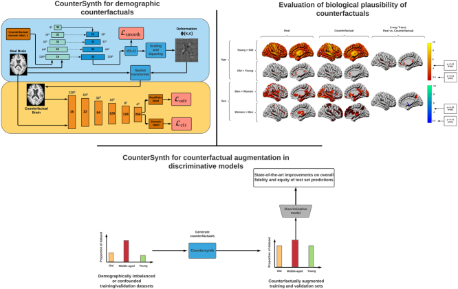
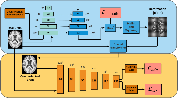
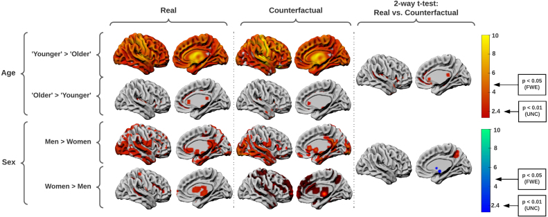
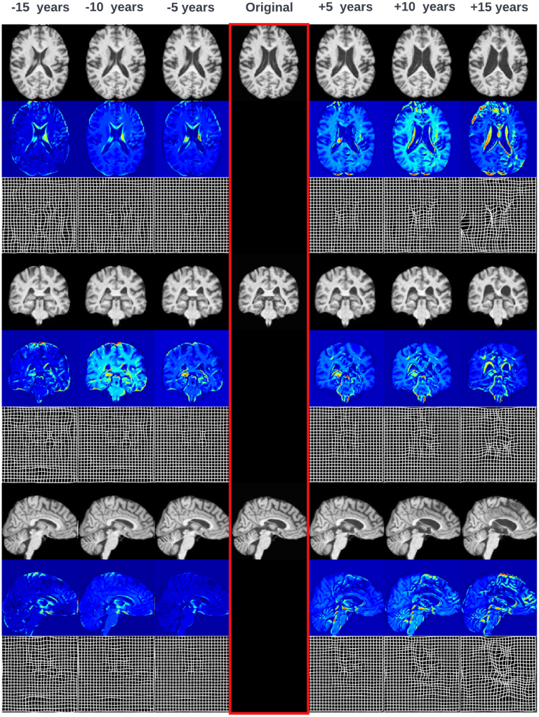
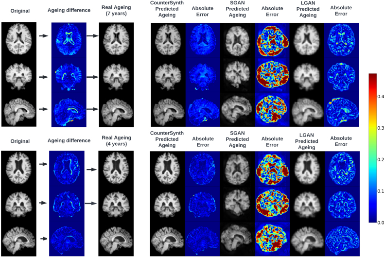
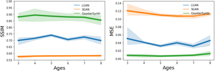
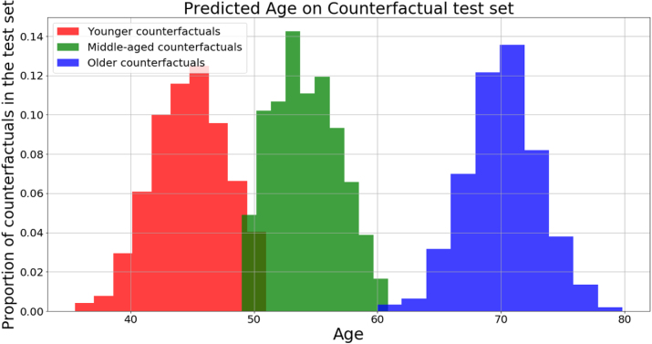
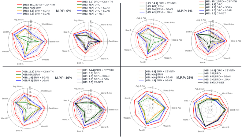
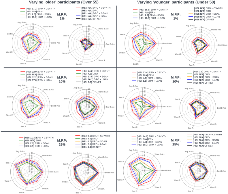
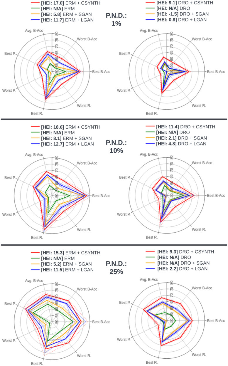
We describe CounterSynth, a conditional generative model of diffeomorphic deformations that induce label-driven, biologically plausible changes in volumetric brain images. The model is intended to synthesise counterfactual training data augmentations for downstream discriminative modelling tasks where fidelity is limited by data imbalance, distributional instability, confounding, or underspecification, and exhibits inequitable performance across distinct subpopulations. Focusing on demographic attributes, we evaluate the quality of synthesised counterfactuals with voxel-based morphometry, classification and regression of the conditioning attributes, and the Fréchet inception distance. Examining downstream discriminative performance in the context of engineered demographic imbalance and confounding, we use UK Biobank and OASIS magnetic resonance imaging data to benchmark CounterSynth augmentation against current solutions to these problems. We achieve state-of-the-art improvements, both in overall fidelity and equity. The source code for CounterSynth is available at https://github.com/guilherme-pombo/CounterSynth.

Keywords: Brain imaging; Counterfactuals; Data augmentation; Deep generative models; Diffeomorphic deformations; Discriminative models; Equity; Fairness.

Graphical abstract

Fig. 1

Top: The U-Net, plus scaling and squaring layers, for predicting and applying the deformation $\mathit{\varphi }$, via the velocity $\mathit{v}$. The input is the real image together with the counterfactual label added as a second image channel. Each block in both pyramids of U-Net layers is a convolutional layer that produces a feature map with $16$, and thereafter $32$, channels. Next to each block is its spatial resolution. These resolutions are decreased with max pooling and increased with nearest neighbour resampling. Dotted arrows represent skip connections. The scaling and squaring block is composed of spatial transformer layers. Bottom: The fully-convolutional discriminator for classifying real and synthesised images. Each upright block is a convolutional layer, producing feature maps with $16,\dots ,256$ channels. Above each block is the spatial resolution. Max pooling is used to reduce this resolution. Two probability distributions are predicted: real vs fake, and a distribution over domain labels.

Fig. 2

SPM’s VBM t-statistics for grey matter changes induced by the CounterSynth age and sex deformations. Leftmost, the grey matter changes associated with age and sex in the original data. Middle, those same changes but in the synthesised counterfactuals. Rightmost, the two one-tailed post-loc t-tests that show voxels where the real and counterfactual regression coefficients differ, the differences being negligible. There are two T-value thresholds to consider, the uncorrected estimation threshold for $p<0.01$ (UNC) and the family-wise estimation threshold for $p<0.05$ (FWE).

Fig. 3

Example synthesis of volumetric counterfactuals for sex and discrete age bins tested on four different participants Age: The first four columns (from left to right) are age counterfactuals. The first three rows show a ‘middle-aged’ brain and its ‘younger’ counterfactual. The last three rows show the ‘older’ counterfactual for a ‘middle-aged’ brain; Sex: Columns five to eight show sex counterfactuals. The first three rows show a ‘female’ brain and its ‘male’ counterfactual. The second three rows show the ‘female’ counterfactual for a ‘male’ brain.

Fig. 4

Example synthesis of continuous age counterfactuals for a single participant. To the left of the original we can see the brain being de-aged in 5 year increments and to the right the brain being aged in 5 year increments. Under each sagittal, coronal and axial slices we show the absolute difference maps between the counterfactual slice and the original one, as well as the displacement fields associated with each transformation. Ageing transformations enlarge the lateral ventricles and expand the size of the sulci. Deageing transformations produce tightened lateral ventricles and sulci. These morphological changes are inline with the ageing deformations described in literature (Sivera et al., 2019, Huizinga et al., 2018).

Fig. 5

Real and predicted ageing for two participants from the OASIS-3 dataset. We present imaging of the participant’s brain at the first collect time point, followed by that same participant’s imaged brain at the final time point, along with associated absolute difference between the two images. Then for each method, we show the predicted brain image for the elapsed time frame (7 and 4 years) alongside with the absolute error between the predicted volume and the ground truth. For easier visual interpretation only the top 50th percentile of the error is shown.

Fig. 6

SSIM (higher is better) and MSE (lower is better) between the real aged brain and the predicted synthesised aged brain for varying amounts of ageing.

Fig. 7

The distribution of predicted ages for the CounterSynth synthesised counterfactuals. Red: Distribution of predicted ages for the ‘middle-aged’ & ‘older’ participants transformed into ‘younger’ participants; Green: Distribution of predicted ages for the ‘younger’ & ‘older’ participants transformed into ‘middle-aged’ participants; black: Distribution of predicted ages for the ‘younger’ & ‘middle-aged’ participants transformed into ‘older’ participants.

Fig. 8

Spider plots depicting the performance of each model in terms of, on separate axes, average balanced accuracy (Avg B-Acc), best subpopulation balanced accuracy (Best B-Acc), worst subpopulation balanced accuracy (Worst B-Acc), best subpopulation precision (Best R.), worst subpopulation precision (Worst R), best subpopulation recall (Best R.), worst subpopulation recall (Worst R.) and, in the legend, the HEI score. The ideal model should be maximal along each axis, yielding an equilateral heptagon shape of maximum surface area, and should exhibit the largest HEI. Dotted lines indicate 1 standard deviation. The minority population percentage (M.P.P.) is manipulated across panels as indicated in the legend. Here we present test set results for sex classification with varying representations of ‘older’ participants. The number of ‘young’ and ‘middle-aged’ patients in the training and validation sets is 5153, 452 respectively. Of the ‘older’ participants in the training and validation sets respectively, 1% amounts to 52, 4 participants, 10% amounts to 572, 50 participants, and 25% amounts to 1717, 151 participants. Here ‘N/A’ indicates that $\Delta L\le 0$ (see Section 2.3), so the HEI does not apply.

Fig. 9

Spider plots depicting the performance of each model in terms of, on separate axes, average balanced accuracy (Avg B-Acc), best subpopulation balanced accuracy (Best B-Acc), worst subpopulation balanced accuracy (Worst B-Acc), best subpopulation precision (Best R.), worst subpopulation precision (Worst R), best subpopulation recall (Best R.), worst subpopulation recall (Worst R.) and, in the legend, the HEI score. The ideal model should be maximal along each axis, yielding an equilateral heptagon shape of maximum surface area, and should exhibit the largest HEI. Dotted lines indicate 1 standard deviation. The minority population percentage (M.P.P.) is manipulated across panels as indicated in the legend. On the left: Test set results for WMH volume classification with varying levels of imbalance for ‘older’ participants. The number of ‘young’ and ‘middle’ patients in the training and validation sets is 5153, 452 respectively. Of the ‘older’ participants in the training and validation sets respectively, 1% amounts to 52, 4 participants, 10% amounts to 572, 50 participants, and 25% amounts to 1717, 151 participants. On the right: Test set results for WMH volume classification with varying levels of imbalance for ‘younger’ participants. The number of ‘older’ patients in the training and validation sets is 6305, 566 respectively. Of the ‘younger’ participants in the training and validation sets respectively, 1% amounts to 64, 6 participants, 10% amounts to 700, 63 participants, and 25% amounts to 2101, 188 participants. Here ‘N/A’ indicates that $\Delta L\le 0$ (see Section 2.3), so the HEI does not apply.

Fig. 10

Spider plots depicting the performance of each model in terms of, on separate axes, average balanced accuracy (Avg B-Acc), best subpopulation balanced accuracy (Best B-Acc), worst subpopulation balanced accuracy (Worst B-Acc), best subpopulation precision (Best R.), worst subpopulation precision (Worst R), best subpopulation recall (Best R.), worst subpopulation recall (Worst R.) and, in the legend, the HEI score. The ideal model should be maximal along each axis, yielding an equilateral heptagon shape of maximum surface area, and should exhibit the largest HEI. Dotted lines indicate 1 standard deviation. The percentage of the natural distribution (P.N.D.) is manipulated across panels as indicated in the legend. Test set results for WMH volume classification with sex and age as collider variables. Here ‘N/A’ indicates that $\Delta L\le 0$ (see Section 2.3), so the HEI does not apply.

References

1. Adeli E., Kwon D., Zhao Q., Pfefferbaum A., Zahr N.M., Sullivan E.V., Pohl K.M. Chained regularization for identifying brain patterns specific to HIV infection. Neuroimage. 2018;183:425–437. - PMC - PubMed
1. Alfaro-Almagro F., Jenkinson M., Bangerter N.K., Andersson J.L., Griffanti L., Douaud G., Sotiropoulos S.N., Jbabdi S., Hernandez-Fernandez M., Vallee E., et al. Image processing and Quality Control for the first 10,000 brain imaging datasets from UK Biobank. Neuroimage. 2018;166:400–424. - PMC - PubMed
1. Arntz R.M., van den Broek S.M., van Uden I.W., Ghafoorian M., Platel B., Rutten-Jacobs L.C., Maaijwee N.A., Schaapsmeerders P., Schoonderwaldt H.C., van Dijk E.J., et al. Accelerated development of cerebral small vessel disease in young stroke patients. Neurology. 2016;87(12):1212–1219. - PMC - PubMed
1. Arsigny V., Commowick O., Pennec X., Ayache N. International Conference on Medical Image Computing and Computer-Assisted Intervention. Springer; 2006. A log-euclidean framework for statistics on diffeomorphisms; pp. 924–931. - PubMed
1. Ashburner J. A fast diffeomorphic image registration algorithm. Neuroimage. 2007;38(1):95–113. - PubMed
Publication types