An official website of the United States government
The .gov means it’s official.
Federal government websites often end in .gov or .mil. Before
sharing sensitive information, make sure you’re on a federal
government site.
The site is secure.
The https:// ensures that you are connecting to the
official website and that any information you provide is encrypted
and transmitted securely.
Identification of structural connections between neurons is a prerequisite to understanding brain function. Here we developed a pipeline to systematically map brain-wide monosynaptic input connections to genetically defined neuronal populations using an optimized rabies tracing system. We used mouse visual cortex as the exemplar system and revealed quantitative target-specific, layer-specific and cell-class-specific differences in its presynaptic connectomes. The retrograde connectivity indicates the presence of ventral and dorsal visual streams and further reveals topographically organized and continuously varying subnetworks mediated by different higher visual areas. The visual cortex hierarchy can be derived from intracortical feedforward and feedback pathways mediated by upper-layer and lower-layer input neurons. We also identify a new role for layer 6 neurons in mediating reciprocal interhemispheric connections. This study expands our knowledge of the visual system connectomes and demonstrates that the pipeline can be scaled up to dissect connectivity of different cell populations across the mouse brain.
J.A.H., K.E.H., P.R.N. and K.N. are currently employed by Cajal Neuroscience. The remaining authors declare no competing interests.
Figures
Extended Data Figure 1.. Comparison of different…
Extended Data Figure 1.. Comparison of different AAV helper viruses and rabies viruses for monosynaptic…
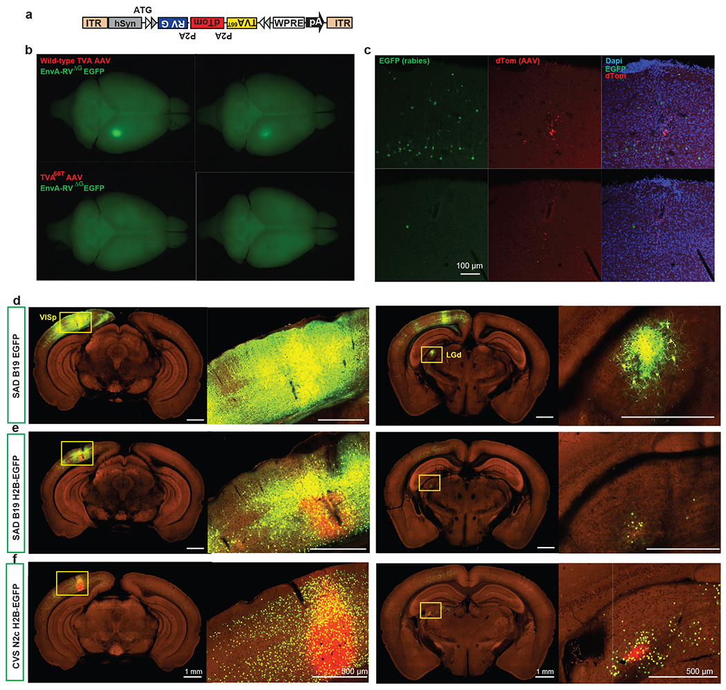
Extended Data Figure 1.. Comparison of different AAV helper viruses and rabies viruses for monosynaptic retrograde tracing.
(a-c) Comparison of spurious rabies infection from AAV helper viruses expressing wild-type TVA and mutant TVA66T. Tricistronic AAV helper viruses were constructed to conditionally express either the wild-type TVA or TVA66T, together with dTomato and RG (a). Cre-negative wild-type mice were sequentially injected with AAV helper viruses and EnvA-pseudotyped recombinant rabies viruses expressing EGFP. Each AAV helper virus/rabies virus pair was tested in two wild-type mice. Top-down view of whole brains (b) and observation of the injection sites under the confocal microscope (c) revealed fewer spurious rabies infection from AAV helper virus expressing TVA66T. (d-f) Comparison of monosynaptic retrograde tracing in VISp using SAD B19 strain of recombinant RV expressing EGFP (d, similar results observed in 6 independent experiments) or H2B-EGFP (e, similar results observed in 7 independent experiments) or CVS N2c strain of recombinant RV expressing H2B-EGFP (f, similar results observed in 303 experiments). Note that in H2B-EGFP expressing SAD B19 experiment there is still green fluorescence in the processes of infected and transmitted neurons (e), due to the very high-level transgene expression in this rabies strain, whereas in CVS N2c experiment H2B-EGFP is strictly contained within nuclei of infected and transmitted neurons (f). Scale bars, 100 μm in b, 1 mm in panels showing full brain sections in d-f, and 500 μm in panels showing selected brain areas in d-f.
Extended Data Figure 2.. Validation of the…
Extended Data Figure 2.. Validation of the AAV helper virus and recombinant rabies used in…
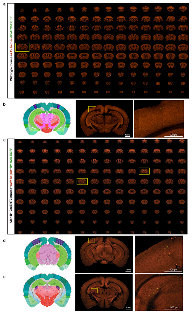
Extended Data Figure 2.. Validation of the AAV helper virus and recombinant rabies used in the retrograde connectomic pipeline in wild-type mice and non-neuronal Cre lines.
(a) Sequential two-photon images of a Cre-negative wild-type mouse brain injected with the AAV helper virus and EnvA-pseudotyped CVS N2cΔG rabies virus expressing H2B-EGFP. Similar results observed in 3 independent experiments. (b) Absence of RV-labeled neurons except a few H2B-EGFP-expressing cells in the injection site. Virus injection was targeted to VISp and validation was conducted in two wild-type mice. Left and middle panels: corresponding 2D atlas plate of Allen CCFv3 and the section image from the outlining box in a showing the injection site. Right panel: Image magnified from the box in the middle panel. Applying the monosynaptic rabies tracing to wild-type mice led to only a few H2B-EGFP-labeled cells in the injection site, but no starter cells in the injection site and no H2B-GFP-labeled cells outside the injection site. This shows that our system does not have the issue of spurious local rabies virus uptake due to low-level expression from the AAV helper in the absence of Cre, or local infection by small quantities of non-pseudotyped, RG-coated RVdG virus particles that may be present in the EnvA-pseudotyped rabies virus preparation. We then confirmed that the trans-synaptic transfer of the recombinant rabies relies on the expression of rabies G from the AAV helper. A G-minus version of the AAV helper virus, which conditionally expresses TVA66T and dTomato after Cre-mediated recombination, was injected into Cre+ mice, followed by the injection of rabies virus three weeks later. We observed H2B-EGFP-labeled cells only at the injection site and nowhere else in the brain. This finding confirms that the presynaptic labeling is specific for the Cre+ starter cells expressing the tricistronic cassette and infected with the RV-H2B-GFP rabies virus. (c) Sequential two-photon images of rabies labeling in an astrocyte-specific Cre mouse brain injected with hSyn promoter-driven AAV helper virus and recombinant rabies virus into VISp. Similar results observed in 4 independent experiments. (d-e) Left and middle two panels: corresponding 2D atlas plates of Allen CCFv3 and the section images from the boxes in c. Right panels: Representative images magnified from the boxes in the middle panels reveal sparse labeling around the injection site (d) and in LGd (e). We tested the monosynaptic rabies tracing system in three non-neuronal Cre lines, Olig2-Cre, Tek-Cre, and Aldh1l1-CreERT2, which express Cre in oligodendrocytes, vascular endothelium, and astrocytes, respectively. Among all experiments using the non-neuronal Cre lines, with either the hSyn-driven AAV helper virus used in the pipeline or a similarly constructed CMV-driven helper virus, sporadic long-distance H2B-EGFP-labeled cells were found only in 50% of the injected Aldh1l1-CreERT2 mice. Our results show that the occasionally infected non-neuronal cells do not support the spread of rabies virus to neurons in local or distant areas.
Extended Data Figure 3.. Overview of experiments…
Extended Data Figure 3.. Overview of experiments included in the final dataset, automatic input signal…
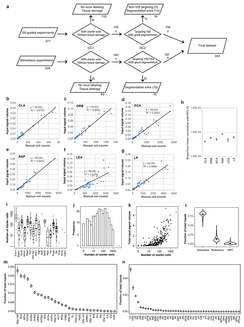
Extended Data Figure 3.. Overview of experiments included in the final dataset, automatic input signal detection and characterization of inputs to cell classes defined by Cre lines in the visual cortex.
(a) Flow chart showing the injection methods, and numbers of experiments passing each QC step. QC1 excluded experiments with no rabies virus labeling or with tissue damage. QC2 excluded experiments with segmentation errors that prevent quantitative analysis or with targeting sites falling outside the visual cortex. One experiment targeting TEa was included in the final data set. For experiments guided by ISI, target validation was performed by overlaying injection polygons with sign maps derived from ISI, and overlaying injection centroids in the CCFv3. Inconsistency between ISI-assigned targets and CCFv3-derived targets were observed in 15 out of the total 136 ISI-guided experiments in the final data set. We assigned injection targets based on the overlaying of injection polygons with sign maps. (b-g) Relationship between per structure input signal volume measured by the informatics data pipeline and manual cell counts. Linear correlation between input signal volume and manually counted input cells was shown in various brain areas. In the six example structures from cortex, thalamus and cortical subplate, strong positive linear correlations were found between automatic measurement and manual counts (R2 in the 0.62-0.98 range). (h) Slopes from linear correlations between informatically measured input signals and manual cell counts in various brain areas. The numbers of independent experiments are as follows: CLA: n=11; ORB: n=10, ACA: n=11, RSP: n=19; LGd: n=19; LP: n=19. (i) Number of starter cells for experiments categorized in Cre lines. Box plots show median and interquartile range (IQR). Whiskers show the largest or smallest value no further than 1.5 × IQR from the hinge. The numbers of independent experiments are as follows: Emx1: n=7, Sepw1: n=19; Cux2: n=29; Nr5a1: n=25; Rbp4: n=25; Tlx3: n=26; A93-Tg1: n=19; Ntsr1: n=21; Ctfg: n=19; Syt6: n=1; Gad2: n=6; Ndnf: n=6; Vip: n=24; Pvalb: n=33; Sst: n=40; Chat: n=1; Htr3a: n=1; Calb1: n=1. (j) Distribution of numbers of starter cells across all experiments. (k) Relationship between numbers of starter cells and total inputs from the whole brain. (l) Fractions of inputs from isocortex, thalamus and HPF to the mouse visual cortex. Dots represent the median values of input signals. (m-n) Fractions of total inputs from non-VIS isocortical areas (m) and thalamic areas (n). Brain areas are ordered according to their levels of input signals. Data are shown as mean ± s.e.m. A total of 303 independent experiments were included.
Extended Data Figure 4.. Representative images of…
Extended Data Figure 4.. Representative images of presynaptic inputs to the visual areas from anatomical…
Extended Data Figure 4.. Representative images of presynaptic inputs to the visual areas from anatomical structures outside of cortex and thalamus.
Coronal STPT images and their corresponding 2D atlas plates in Allen CCFv3 show labeled presynaptic neurons in OLF (a-a”), HPF (b-b”), CTXsp (c-c”), STR (d-c”), PAL (e-e”), HY (f-f”), MB (g-g”), pons (h-h”), and MY (i-i”). Claustrum (CLA) in CTXsp, diagonal band nucleus (NDB) in PAL, and lateral hypothalamic area (LHA) in HY each represent ~0.1% of whole brain inputs; globus pallidus, external segment (GPe) in PAL, basolateral amygdalar nucleus (BLA) in CTXsp, and zona incerta (ZI) in HY each account for ~0.01% of whole brain inputs; dorsal peduncular area (DP) in OLF, locus ceruleus (LC) in pons, and superior colliculus (SC) in MB each account for ~0.001% of whole brain inputs; areas in MY each account for ~0.0001% of whole brain inputs. Rare inputs in several structures of MY are also found in less than 10% of all experiments (Supplementary Table 3), which could be missed using other connectivity mapping techniques. Clustered inputs are found in NDB (fraction of whole brain inputs in NDB > 0 in 93% of all experiments), substantia innominata (SI) (fraction of whole brain inputs in SI > 0 in 75% of all experiments), LC (fraction of whole brain inputs in LC > 0 in 66% of all experiments), and DR (~0.01% of whole brain inputs, found in 63% of all experiments). The numbers of independent experiments with similar results are 121 in a, 61 in a’, 52 in a”, 254 in b, 165 in b’, 137 in b”, 278 in c, 187 in c’, 149 in c”, 236 in d, 187 in d’, 68 in d”, 226 in e, 110 in e’, 152 in e”, 275 in f, 224 in f’, 198 in f”, 214 in g, 187 in g’, 33 in g”, 231 in h, 193 in h’, 193 in h”, 53 in i, 52 in i’, and 30 in i”. Enlarged views of boxed areas are shown in the right-hand panels for each major brain structure. Arrows highlight the location of single labeled cells.
Extended Data Figure 5.. Connectivity matrices comparing…
Extended Data Figure 5.. Connectivity matrices comparing the inputs to Rbp4 (a) and Sst (b)…
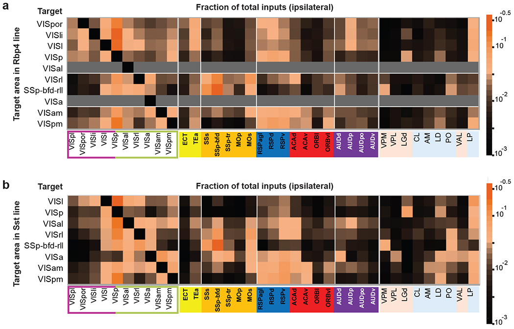
Extended Data Figure 5.. Connectivity matrices comparing the inputs to Rbp4 (a) and Sst (b) neurons in the visual areas from within the visual cortex, non-visual isocortical modules, and thalamus.
Gray indicates experiments not available. In the matrix, each row represents experiments with the same target area, and each cell shows the fraction of the total inputs in a given input structure measured from a single experiment or the average when n > 1.
Extended Data Figure 6.. Brain-wide input patterns…
Extended Data Figure 6.. Brain-wide input patterns to excitatory neuron subclasses in different layers of…
Extended Data Figure 6.. Brain-wide input patterns to excitatory neuron subclasses in different layers of the primary visual cortex.
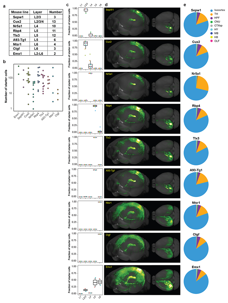
(a-b) Overview of the layer selectivity and number of experiments of each transgenic Cre line (a) and the numbers of starter cells grouped by Cre lines (b) for the 48 experiments in VISp. (c) Laminar distribution of starter cells for each Cre line. For each transgenic line, different experiments are indicated by different colors. Box plots show median and interquartile range (IQR). Whiskers show the largest or smallest value no further than 1.5 × IQR from the hinge. The numbers of independent experiments are as follows: Sepw1: n=3; Cux2: n=13; Nr5a1: n=10; Rbp4: n=11; Tlx3: n=12; A93-Tg1: n=6; Ntsr1: n=4; Ctfg: n=3; Emx1: n=2. (d) Representative 3D visualization of brain-wide inputs to neurons in different layers of VISp. (e) Brain-wide input patterns of major brain structures to different layer-specific excitatory neuron subclasses labeled by Cre lines.
Extended Data Figure 7.. Comparison of subcortical…
Extended Data Figure 7.. Comparison of subcortical inputs to excitatory neurons in different layers of…
Extended Data Figure 7.. Comparison of subcortical inputs to excitatory neurons in different layers of VISp and brain-wide input patterns to excitatory neuron subclasses in VISl.
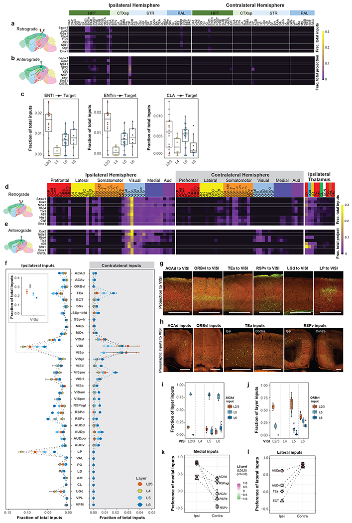
(a) Connectivity matrix showing presynaptic inputs from the ipsilateral and contralateral HPF, CTXsp, STR, and PAL to excitatory neurons in different layers of VISp. Each row of the matrix represents the mean per structure fraction of total input signals for experiments in each Cre line. Rows are organized based on layer-specific distribution of the starter cells. Brain regions are ordered by ontology order in the Allen CCFv3. (b) Connectivity matrix showing normalized projections from VISp to the brain regions shown in (a). Anterograde tracing experiments (Supplementary Table 4) from the Cre mouse lines used in (a) and C57BL/6J were included, and rows represent the mean per structure fraction of total projection signals for experiments in each mouse line. (c) Comparison of ENTl, ENTm, and CLA inputs to excitatory neurons in different layers of VISp. Box plots show median and interquartile range (IQR). Whiskers show the largest or smallest value no further than 1.5 × IQR from the hinge (same below). The numbers of independent experiments are as follows: L2/3: n=16; L4: n=10; L5: n=29; L6: n=7. (d) Connectivity matrix showing normalized inputs from the ipsilateral and contralateral isocortex, and ipsilateral thalamus to excitatory neurons in different layers of VISl. Each row of the matrix represents the mean per structure fraction of total input signals for experiments in each Cre line. Rows are organized based on layer-specific distribution of the starter cells. The cortical areas are ordered first by module membership (color coded) then by ontology order in the Allen CCFv3. The ten thalamic nuclei are ordered based on the strength of inputs, and are color coded by the thalamocortical projection classes (blue: core, green: intralaminar, brown: matrix-focal, and red: matrix-multiareal). (e) Connectivity matrix showing normalized axon projections from VISl to the ipsilateral and contralateral isocortex, and ipsilateral thalamus shown in (d). Anterograde tracing experiments (Supplementary Table 5) from the Cre mouse lines used in (d) and C57BL/6J were included, and rows represent the mean per structure fraction of total projection signals for experiments in each mouse line. (f) Comparison of inputs from ipsilateral and contralateral cortical areas and thalamic nuclei to excitatory neurons in different layers of VISl. The inset shows fraction of inputs from VISp to excitatory neurons in different layers of VISl. Data are shown as mean ± s.e.m. The numbers of independent experiments are as follows: L2/3: n=5; L4: n=4; L5: n=11; L6: n=8. (g-h) Representative STPT images showing laminar termination patterns of axon projections in VISl from higher-order association cortical areas and thalamic nuclei (g) and laminar distribution patterns of presynaptic input cells in the cortical areas that project to VISl (h). Ipsi, ipsilateral hemisphere. Contra, contralateral hemisphere. (i-j) Quantification of laminar distribution of inputs from ACAd (i, numbers of independent experiments: L2/3: n=3; L5: n=10; L6: n=7) and ORBvl (j, numbers of independent experiments: L2/3: n=2; L5: n=11; L6: n=7) to excitatory neurons in different layers of VISl. The fraction of layer inputs is calculated as the fraction of the total input signals in a given source area across layers. (k-l) Comparison of L5 and L6 preference for medial (k) or lateral (l) source cortical areas in the ipsilateral and contralateral hemispheres sending presynaptic inputs to VISl. The preference score for a given cortical area is calculated as (L5 input - L6 input) / (L5 input + L6 input). Each source cortical area was colored according to its preference score. Data are shown as mean ± s.e.m. The numbers of independent experiments included are as follows: ACAd (Ipsi): n=35; ACAv (Ipsi): n=26; RSPd (Ipsi): n=40; RSPv (Ipsi): n=43, RSPagl (Ipsi): n=36, AUDp (Ipsi): n=39, AUDv (Ipsi): n=30; TEa (Ipsi): n=42, ECT (Ipsi): n=30, ACAd (Contra): n=8; ACAv (Contra): n=4; RSPd (Contra): n=14; RSPv (Contra): n=10, RSPagl (Contra): n=13, AUDp (Contra): n=17, AUDv (Contra): n=13; TEa (Contra): n=26, ECT (Contra): n=14. Scale bars, 500 μm. We also find generally consistent input patterns to excitatory neurons in different layers of other HVAs as of VISp and VISl, though due to smaller number of experiments in each layer of each region (Figure 2a) we do not provide quantitative analysis here.
Extended Data Figure 8.. Comparison of contralateral…
Extended Data Figure 8.. Comparison of contralateral cortical inputs to excitatory neuron subclasses in different…
Extended Data Figure 8.. Comparison of contralateral cortical inputs to excitatory neuron subclasses in different layers of visual areas.
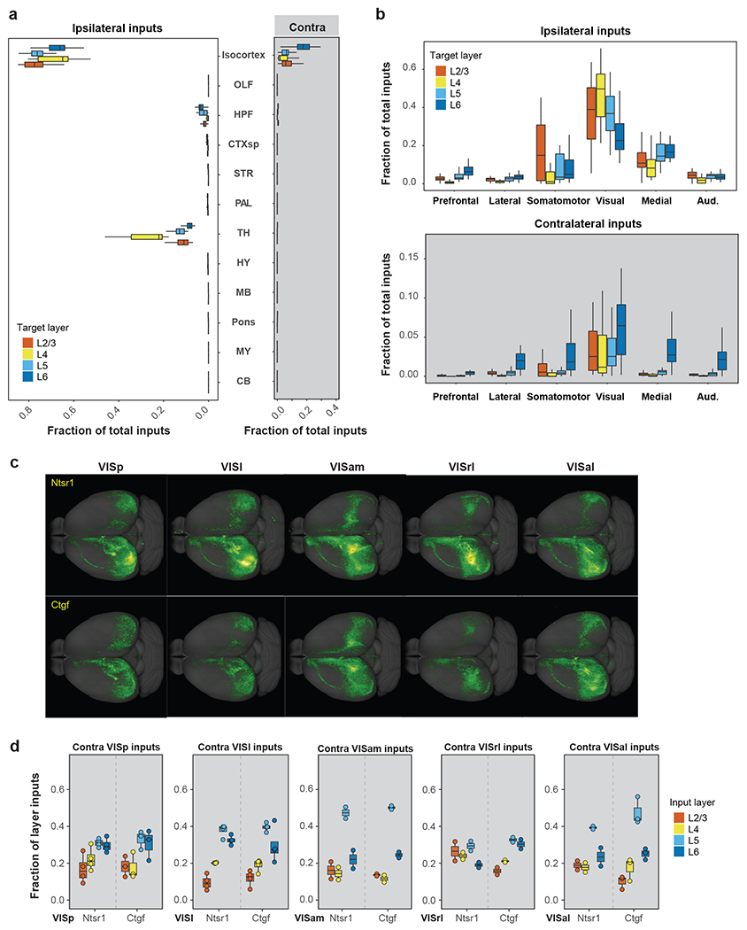
(a) Comparison between ipsilateral (left) and contralateral (right) brain-wide inputs to excitatory neuron subclasses with starter cells restricted to either L2/3, L4, L5 or L6 of visual areas. A total of 89 experiments with starter cells restricted in a single layer were identified, and the target areas included both VISp and HVAs. (b) Comparison between ipsilateral (top) and contralateral (bottom) isocortical inputs for each cortical module to excitatory neuron subclasses with starter cells restricted to either L2/3 (n=20 numbers of independent experiments), L4 (n=18 numbers of independent experiments), L5 (n=25 numbers of independent experiments) or L6 (n=27 numbers of independent experiments) of visual areas. (c) Representative top-down view of inputs to Ntsr1 and Ctgf Cre line-labeled L6 and L6b cell types in visual areas. (d) Laminar distribution of presynaptic inputs from the homotypic contralateral areas to Ntsr1 and Ctgf Cre line-labeled neurons in visual areas shown in (c). The fraction of layer inputs is calculated as the fraction of the total input signals in a given source area across layers. L1 is excluded from the analysis due to overall lack of signal in this layer. Box plots show median and interquartile range (IQR). Whiskers show the largest or smallest value no further than 1.5 × IQR from the hinge. The numbers of independent experiments are as follows: Ntsr1 in VISp: n=4; Ctgf in VISp: n=3; Ntsr1 in VISl: n=4; Ctgf in VISl: n=4; Ntsr1 in VISam: n=2; Ctgf in VISam: n=2; Ntsr1 in VISrl: n=2; Ctgf in VISrl: n=2; Ntsr1 in VISal: n=2; Ctgf in VISal: n=3.
Extended Data Figure 9.. Analysis of brain-wide…
Extended Data Figure 9.. Analysis of brain-wide input patterns to interneuron subclasses in VISp, and…
Extended Data Figure 9.. Analysis of brain-wide input patterns to interneuron subclasses in VISp, and comparison of local inputs to excitatory neurons in different layers of VISl.
(a) Summary of the numbers of starter cells for each interneuron subclass. Each dot represents one individual experiment. (b) Laminar distribution of starter cells for each interneuron subclass. For each transgenic line, different experiments are indicated by different colors. Box plots show median and interquartile range (IQR). Whiskers show the largest or smallest value no further than 1.5 × IQR from the hinge (same below). The number of independent experiments included are as follows: Gad2: n=2; Ndnf: n=2; Pvalb: n=9; Sst: n=17; Vip: n=9. (c) Representative 3D visualization of brain-wide inputs to interneuron subclasses in VISp. (d) Overview of brain-wide inputs to different interneuron subclasses. (e-h) Layer-specific inputs of ipsilateral VISl to excitatory neurons in L2/3 (e, n=5 independent experiments), L4 (f, n=4 independent experiments), L5 (g, n=11 independent experiments) and L6 (h, n=8 independent experiments) of VISl and representative images of local VISl inputs. Starter cells are identified by the co-expression of dTomato from the AAV helper virus and nucleus-localized H2B-EGFP from the rabies virus.
Extended Data Figure 10.. Comparison of laminar…
Extended Data Figure 10.. Comparison of laminar distribution of visual inputs to SSp-bfd-rll (a-b) and…
Extended Data Figure 10.. Comparison of laminar distribution of visual inputs to SSp-bfd-rll (a-b) and VISrl (c-d).
(a, c) Laminar distribution of inputs from various visual areas to SSp-bfd-rll (a, the numbers of independent experiments are: VISli and VISpm: n=5, VISl and VISa: n=12; VISp, VISal, and VISrl: n=13; VISam: n=7) and VISrl (c, the numbers of independent experiments are: VISli and VISpm: n=20, VISl and VISa: n=21; VISp: n=23; VISal and VISrl: n=22; VISam: n=19). Box plots show median and interquartile range (IQR). Whiskers show the largest or smallest value no further than 1.5 × IQR from the hinge. (b, d) Representative images of inputs from VISp, VISpm and VISal to SSp-bfd-rll (b) and VISrl (d).
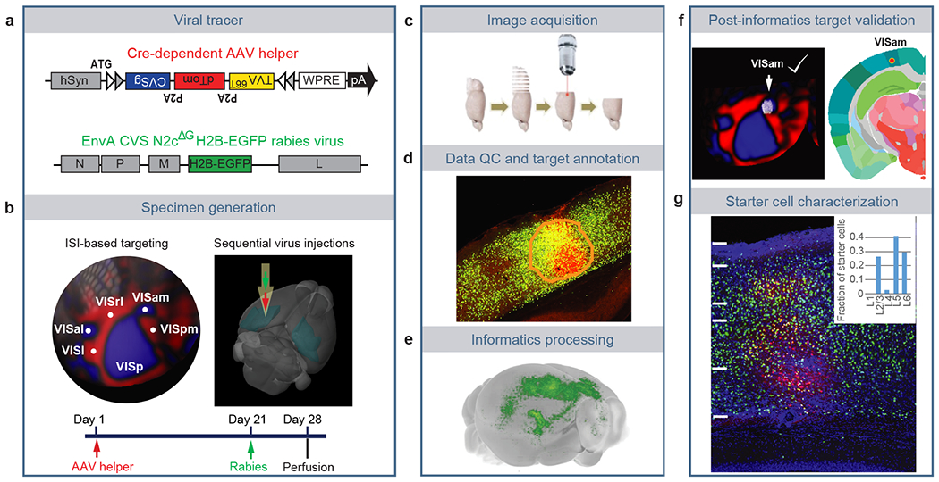
Figure 1.. Pipeline identifying monosynaptic inputs to specific neuronal populations in the visual cortex.
( …
Figure 1.. Pipeline identifying monosynaptic inputs to specific neuronal populations in the visual cortex.
(a) Viral tools for mapping monosynaptic inputs to Cre-expressing neurons. The tricistronic AAV helper virus conditionally expresses TVA66T, dTomato, and rabies glycoprotein of the CVS N2c strain (CVSg) after Cre-mediated recombination. The EnvA-pseudotyped CVS N2cΔG rabies virus expresses histone-EGFP (H2B-EGFP) from the rabies G gene locus in the recombinant rabies virus genome. (b) ISI-based targeting, stereotaxic injection, and experimental timeline for virus injections and brain collection. (c) Sequential two-photon images were acquired at 100 μm interval and a total of 140 images were obtained for each brain. (d) Target sites were annotated by drawing injection polygons based on the expression of dTomato from the AAV helper virus. (e) Image series was automatically segmented and registered into the Allen CCFv3. (f) Injection site was verified post hoc by overlaying the injection site detected by AAV helper expression with an ISI image, and/or by overlaying the injection centroid to CCFv3. (g) Starter cell characterization. Sections around the planned injection site were collected and dTomato signal was enhanced by immunostaining. Starter cells were then detected by co-expression of dTomato and nuclear EGFP, and layer-distribution of the starter cells was analyzed.
Figure 2.. Identification of monosynaptic inputs to…
Figure 2.. Identification of monosynaptic inputs to Cre-labeled neuronal classes in different visual areas.
(a) …
Figure 2.. Identification of monosynaptic inputs to Cre-labeled neuronal classes in different visual areas.
(a) Summary of Cre mouse lines, target areas, and numbers of the 303 experiments in the visual areas. The injection target areas were verified based on overlay of injection site polygons with ISI images and/or the position of injection site polygons in Allen CCFv3. (b) Mapping of each injection centroid in the cortical flat map (with six cortical modules labeled: prefrontal, lateral, somatomotor, visual, medial and auditory). Color indicates different visual areas. Twelve injections were performed into the right hemisphere, the remaining 291 injections were performed into the left hemisphere, and injection site was verified post-hoc. Locations of all injection centroids were plotted onto the CCFv3 cortical flat map, with the right hemisphere injection centroids flipped to their corresponding sites in the left hemisphere for comparative analysis. (c) Connectivity matrix showing normalized inputs from the ipsilateral and contralateral hemispheres for all experiments. Each row represents a single experiment. Columns are ordered by 12 major brain divisions; rows are organized according to hierarchical clustering of the input patterns. The input signal per structure was measured by the informatics data pipeline and represented by per structure input signal volume (sum of detected signal in mm3) after thresholding to minimize false positive signals (see Methods), and then normalized to the total inputs of the whole brain. Value in each cell of the matrix represents the input signal volume in the given brain area as the fraction of total inputs of the brain. Color in the “Target” represents the verified injection target area of the experiment in each row, as color-coded in (b).
Figure 3.. Comparison of brain-wide inputs to…
Figure 3.. Comparison of brain-wide inputs to neurons in the primary visual cortex and higher…
Figure 3.. Comparison of brain-wide inputs to neurons in the primary visual cortex and higher visual areas.
(a) Comparison of whole-brain inputs to the visual areas. Inputs from isocortex were divided into six modules. Numbers of independent experiments for each target are in Figure 2a. Box plots show median and interquartile range (IQR). Whiskers show the largest or smallest value no further than 1.5 × IQR from the hinge. Somo, somatomotor. OLF, olfactory areas. HPF, hippocampal formation. CTXsp, cortical subplate. STR, striatum. PAL, pallidum. TH, thalamus. HY, hypothalamus. MB, midbrain. MY, medulla. CB, cerebellum. (b-d) Matrices showing inputs to visual area targets from top input areas. Each cell represents the average value of fraction of total inputs from a given input area in all the experiments for a given target. Visual input areas are separated into dorsal and ventral streams and ordered based on their hierarchical organization. Non-visual input cortical areas are grouped by module membership. Input thalamic areas are ordered by previously predicted hierarchical orders. Areas in the sensory-motor cortex related or polymodal association cortex related part of thalamus are highlighted in pink or blue, respectively. (e) Matrix showing Spearman’s R between experiments within the same target (intra-target, mean of Rs between experiments of different Cre lines) and between experiments across different targets (inter-target, mean of Rs between experiments of same Cre line in different targets). (f) Frequency distributions of intra-target and inter-target Spearman’s R. A curve was fit to each distribution. (g) Comparison of inputs between VISrl (Rbp4: n=1, Sst: n=2) and VISpm (Rbp4: n=2, Sst: n=3). (h) Comparison of LGd, LP and SCs inputs to VISpor in 14 experiments. Each symbol represents one experiment. (i) Example of a Cux2-IRES-Cre VISpor experiment. Two independent experiments led to similar results. Left: Injection centroid mapped to VISpor in Allen CCFv3. Middle: Brain section containing the injection site and labeling in SCs. Right: Confocal image of the injection site and labeling in LGd and LP.
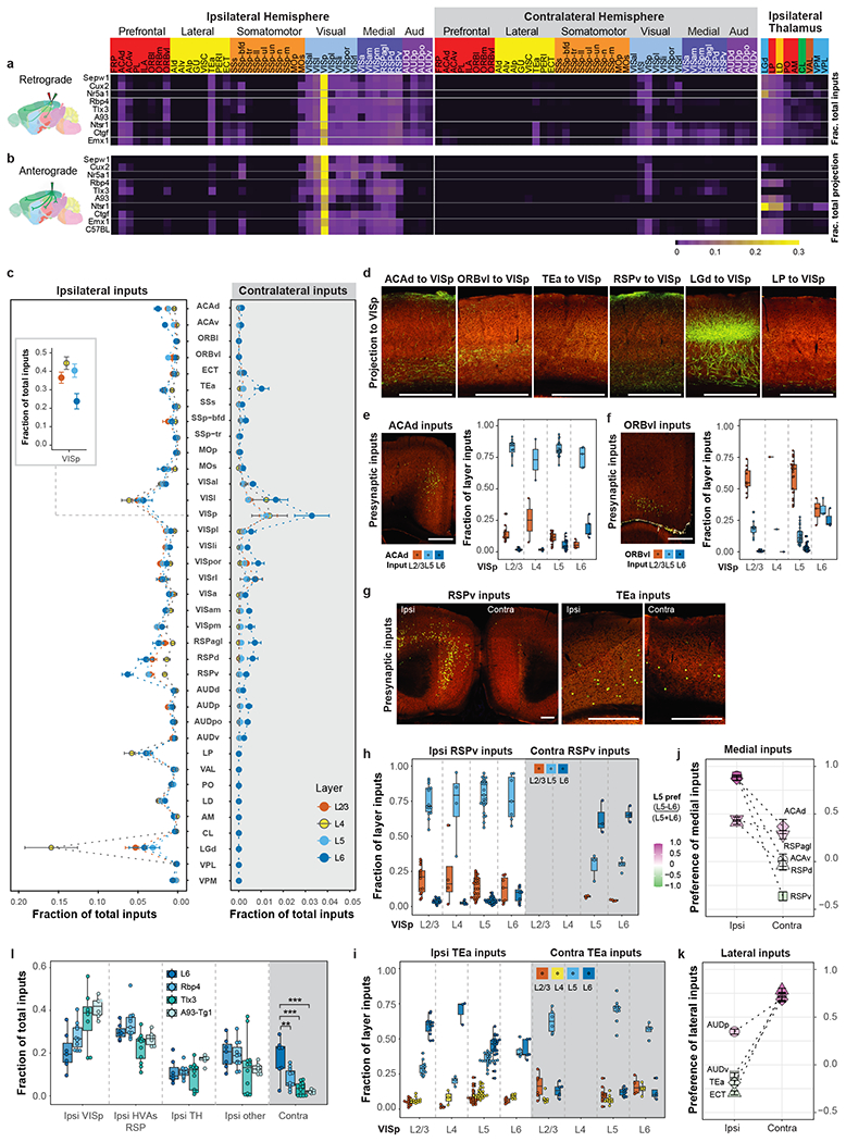
Figure 4.. Comparison of brain-wide input patterns…
Figure 4.. Comparison of brain-wide input patterns to excitatory neuron subclasses in different layers of…
Figure 4.. Comparison of brain-wide input patterns to excitatory neuron subclasses in different layers of the primary visual cortex.
(a-b) Matrix showing inputs from the isocortex and thalamus to excitatory neurons in different layers of VISp (a) and matrix showing the reciprocal axonal projections from VISp (b). Each row represents the mean fraction of total input or projection signals per structure in each mouse line. Cortical module memberships and thalamocortical projection classes (blue: core, green: intralaminar, brown: matrix-focal, and red: matrix-multiareal) are color-coded. (c) Comparison of inputs to excitatory neurons in different layers of VISp (independent experiments: 16, 10, 29 and 7 for L2/3, L4, L5 and L6, respectively). Data are shown as mean ± s.e.m. The inset shows local VISp inputs. (d) Laminar termination patterns of axon projections in VISp from source areas (ACAd: n=3; ORBvl: n=2; TEa, n=1; RSPv: n=2; LGd: n=5; and LP: n=1). (e-i) Laminar distribution pattern of input cells in ACAd, ORBvl, RSPv and TEa projecting to excitatory neurons in VISp. The fraction of layer inputs is calculated as the fraction of the total input signals in a given source area across layers. L1 is excluded from the analysis due to overall lack of signal in this layer. Independent experiments: e, 11, 2, 21 and 5 for L2/3, L4, L5 and L6, respectively; f, 10, 1, 24, 3 for L2/3, L4, L5 and L6, respectively; RSPv in g,h: Ipsi: 14, 4, 25, and 7 for L2/3, L4, L5 and L6, respectively; Contra: 3, and 4 for L5 and L6 respectively; TEa in g,i: Ipsi: 12, 3, 24, and 5 for L2/3, L4, L5 and L6, respectively; Contra: 6, 10 and 4 for L2/3, L5 and L6, respectively. (j-k) Comparison of L5 and L6 preference for medial (j) or lateral (k) source cortical areas sending inputs to VISp. A preference score for a given cortical area (L5 input - L6 input) / (L5 input + L6 input) shows that ipsilateral inputs to VISp come preferentially from L5 of medial areas and L6 of lateral areas, whereas contralateral inputs to VISp present an opposite bias. Data are shown as mean ± s.e.m. Independent experiments: Ipsi: ACAd: n=56; ACAv: n=40; RSPd: n=73; RSPv: n=78, RSPagl: n=61, AUDp: n=56, AUDv: n=43; TEa: n=65, ECT: n=37; Contra: ACAd: n=9; ACAv: n=8; RSPd: n=17; RSPv: n=12, RSPagl: n=16, AUDp: n=14, AUDv: n=10; TEa: n=27, ECT: n=11. (l) Comparison of inputs to L6 and different L5 cell populations in VISp (L6: n=7; Rbp4: n=11; Tlx3: n=12; A93-Tg1: n=6). **p < 0.01, ***p < 0.001. Tukey multiple comparisons of means: L6 vs Rbp4: p=0.0015, L6 vs Tlx3: p=0.000004, L6 vs A93-Tg1: p=0.000015. Box plots show median and interquartile range (IQR). Whiskers show the largest or smallest value no further than 1.5 × IQR from the hinge. Scale bars, 500 μm.
Figure 5.. Comparison of brain-wide input patterns…
Figure 5.. Comparison of brain-wide input patterns to different interneuron subclasses in the primary visual…
Figure 5.. Comparison of brain-wide input patterns to different interneuron subclasses in the primary visual cortex.
(a) Frequency distribution of Spearman’s R values for brain-wide input patterns to different excitatory neuron (EN) subclasses, those to different interneuron (IN) subclasses, and Rs measured between EN input patterns and IN input patterns. (b) Comparison of ipsilateral (left) and contralateral (right) inputs from the visual and medial cortical modules and thalamus to EN and IN cell classes located in the VISl (square), VISp (circle), and VISam (diamond). The numbers of EN experiments are 64 for VISp, 30 for VISl, and 14 for VISam. The numbers of IN experiments are 39 for VISp, 26 for VISl, and 12 for VISam. Data are shown as mean ± s.e.m. (c) Comparison of ipsilateral cortical inputs and thalamic inputs to Sst (n=17), Pvalb (n=9) and Vip (n=9) cells in VISp. Data are shown as mean ± s.e.m. (d) Heatmap of starter cell layer distribution for the 39 interneuron experiments in VISp separating experiments into different depth groups. (e) Comparison of inputs from ipsilateral and contralateral cortical areas and thalamic nuclei to interneuron groups located in different depths of VISp. The numbers of independent experiments included are as follows: Top: n=5, Upper: n=10; Lower: n=16; Bottom: n=8. Data are shown as mean ± s.e.m. (f) Comparison of contralateral cortical inputs between the Bottom group and various interneuron subclasses. The numbers of independent experiments included are as follows: Bottom: n=8; Sst: n=17, Pvalb: n=9; Vip: n=9; Ndnf: n=2, Gad2: n=2. Data are shown as mean ± s.e.m. Independent two sample t test (two-sided), **p < 0.01, *p < 0.05, Bottom vs Sst: p=0.018, Bottom vs Vip: p=0.017, Bottom vs Ndnf: p=0.0030, and Pvalb vs Ndnf: p=0.016.
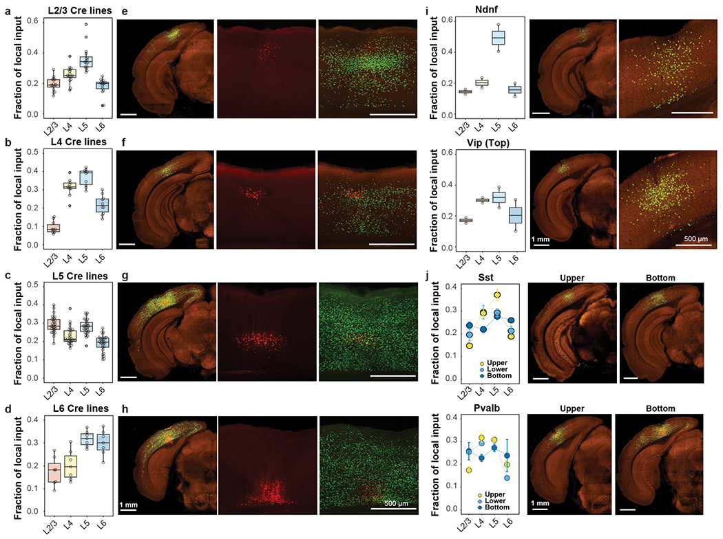
Figure 6.. Comparison of local inputs to…
Figure 6.. Comparison of local inputs to excitatory neurons and inhibitory interneurons in different depths…
Figure 6.. Comparison of local inputs to excitatory neurons and inhibitory interneurons in different depths of the primary visual cortex.
(a-d) Layer-specific inputs of ipsilateral VISp to excitatory neurons in L2/3 (a, n=16 independent experiments), L4 (b, n=10 independent experiments), L5 (c, n=29 independent experiments) and L6 (d, n=7 independent experiments) of VISp. (e-h) Representative images showing layer-specific local inputs to excitatory neurons in L2/3 (e), L4 (f), L5 (g) and L6 (h) of VISp. Left panels show STPT images of brain sections containing starter cells, and right two panels are confocal microscopic images showing the distribution of starter cells and local inputs. Starter cells are identified by the co-expression of dTomato from the AAV helper virus and nucleus-localized H2B-EGFP from the rabies virus. (i) Comparison of local input patterns to Ndnf-Cre and Vip-Cre experiments with Top distribution of starter cells (Ndnf and Vip: n=2 independent experiments). (j) Comparison of local inputs to Sst and Pvalb experiments with different depths of starter cell distribution. Representative images containing the injection sites are provided for Sst-Cre and Pvalb-Cre experiments in the Upper and Bottom groups. The numbers of independent Sst-Cre experiments in the Upper, Lower, and Bottom groups are 2, 10, and 4, respectively, and those of Pvalb experiments in the Upper, Lower, and Bottom groups are 6, 1, and 2, respectively. Data are shown as mean ± s.e.m. Box plots show median and interquartile range (IQR). Whiskers show the largest or smallest value no further than 1.5 × IQR from the hinge.
Figure 7.. Relative hierarchical positions of the…
Figure 7.. Relative hierarchical positions of the primary visual cortex and higher visual areas.
(a) …
Figure 7.. Relative hierarchical positions of the primary visual cortex and higher visual areas.
(a) Laminar distribution of inputs for connections between VISp and VISam. Mean fraction of layer-specific inputs between the source area and the target area was used. (b-c) Comparison of laminar distribution of visual area inputs to VISp (b, n=103 independent experiments) and VISam (c, n=26 independent experiments). Each dot represents the mean (± s.e.m.) fraction of layer-specific inputs. . Arrows indicate ascending order of hierarchical positions of the dorsal and ventral streams. (d-f) Comparison of the fraction of layer-specific inputs from various cortical areas (colored according to the mean fraction of inputs) to VISp. (g) Matrix of h index of inputs from the 10 visual areas to the 9 targets. Each cell represents the mean h index of inputs in a given source area to a target area. Light gray denotes no availability of data. (h) Pairs plots showing the correlation of measured h index values of cortical source areas sending inputs to specific pairs of target areas. Each point represents the average pair of h index values obtained in a given source area to a pair of target areas. Red lines are the best fit lines (least-squares regression lines), and blue lines are the lines with a slope equal to 1 that best fit the points. (i) Correlation between measured and predicted h index values between cortical source areas and the five target visual areas in panel h. (j) Estimated hierarchical levels obtained by the linear regression model. The hierarchical level of VISp was set at zero. Error bars indicate 90% confidence intervals, with centrers representing the predicted hierarchical values for other visual areas. Visual areas are separated into the dorsal and ventral streams (to the right and left of VISp, respectively). Numbers of independent experiments: VISl: n=56, VISp: n=103, VISal: n=20, VISrl: n=23, and VISam: n=26.
Callaway EM Transneuronal circuit tracing with neurotropic viruses. Current opinion in neurobiology 18, 617–623, doi:10.1016/j.conb.2009.03.007 (2008).
-
DOI
-
PMC
-
PubMed
Callaway EM & Luo L Monosynaptic Circuit Tracing with Glycoprotein-Deleted Rabies Viruses. J Neurosci 35, 8979–8985, doi:10.1523/JNEUROSCI.0409-15.2015 (2015).
-
DOI
-
PMC
-
PubMed
Beier KT et al. Rabies screen reveals GPe control of cocaine-triggered plasticity. Nature 549, 345–350, doi:10.1038/nature23888 (2017).
-
DOI
-
PMC
-
PubMed
Kim EJ, Jacobs MW, Ito-Cole T & Callaway EM Improved Monosynaptic Neural Circuit Tracing Using Engineered Rabies Virus Glycoproteins. Cell reports 15, 692–699, doi:10.1016/j.celrep.2016.03.067 (2016).
-
DOI
-
PMC
-
PubMed
Lo L & Anderson DJ A Cre-dependent, anterograde transsynaptic viral tracer for mapping output pathways of genetically marked neurons. Neuron 72, 938–950, doi:10.1016/j.neuron.2011.12.002 (2011).
-
DOI
-
PMC
-
PubMed
Methods-only references:
Gorski JA et al. Cortical excitatory neurons and glia, but not GABAergic neurons, are produced in the Emx1-expressing lineage. J Neurosci 22, 6309–6314, doi:20026564 (2002).
-
PMC
-
PubMed
Franco SJ et al. Fate-restricted neural progenitors in the mammalian cerebral cortex. Science (New York, N.Y 337, 746–749, doi:10.1126/science.1223616 (2012).
-
DOI
-
PMC
-
PubMed
Dhillon H et al. Leptin directly activates SF1 neurons in the VMH, and this action by leptin is required for normal body-weight homeostasis. Neuron 49, 191–203, doi:10.1016/j.neuron.2005.12.021 (2006).
-
DOI
-
PubMed
Gerfen CR, Paletzki R & Heintz N GENSAT BAC cre-recombinase driver lines to study the functional organization of cerebral cortical and basal ganglia circuits. Neuron 80, 1368–1383, doi:10.1016/j.neuron.2013.10.016 (2013).
-
DOI
-
PMC
-
PubMed
Daigle TL et al. A Suite of Transgenic Driver and Reporter Mouse Lines with Enhanced Brain-Cell-Type Targeting and Functionality. Cell 174, 465–480 e422, doi:10.1016/j.cell.2018.06.035 (2018).
-
DOI
-
PMC
-
PubMed