GeoSPM: Geostatistical parametric mapping for medicine

Abstract

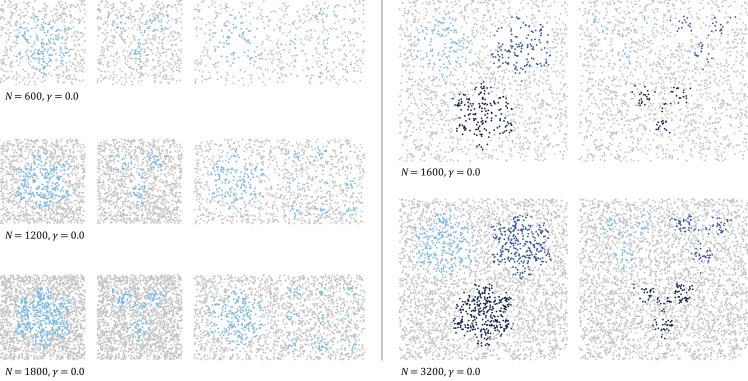
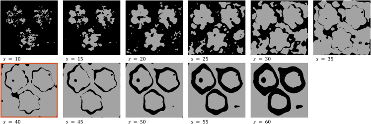
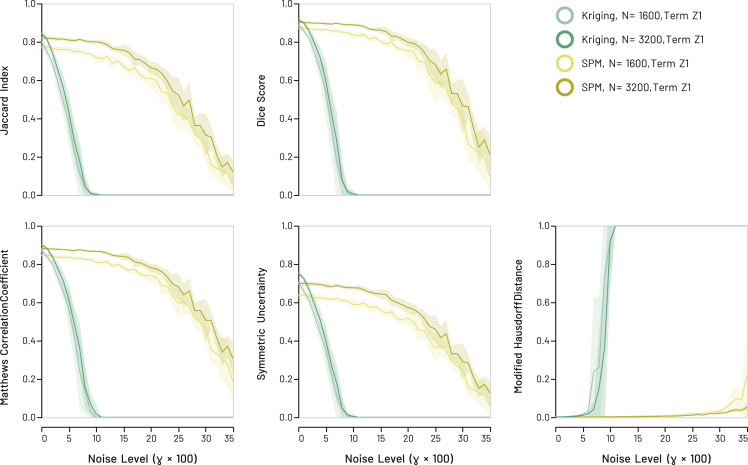
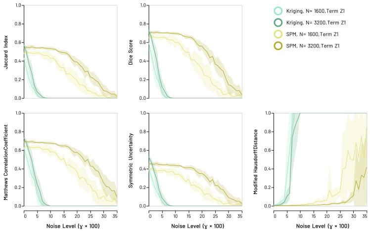
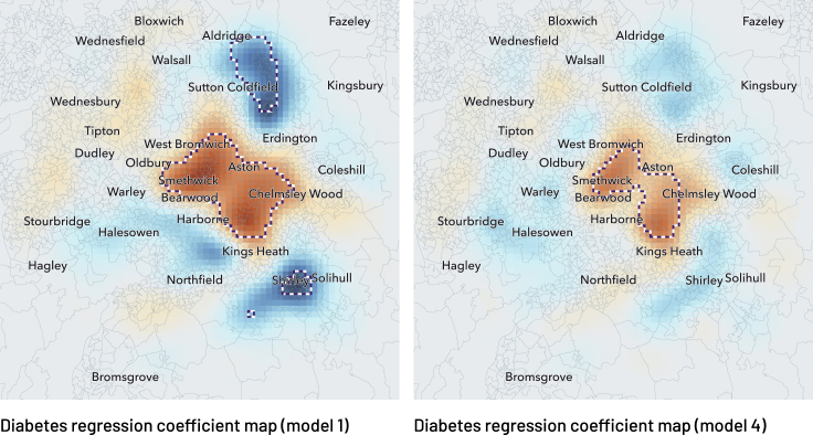
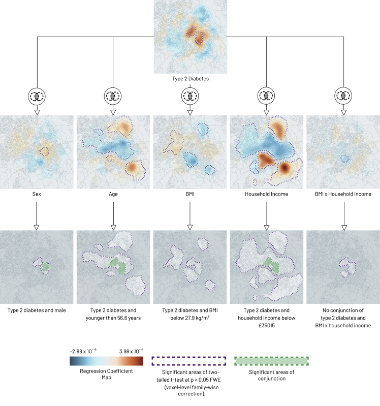
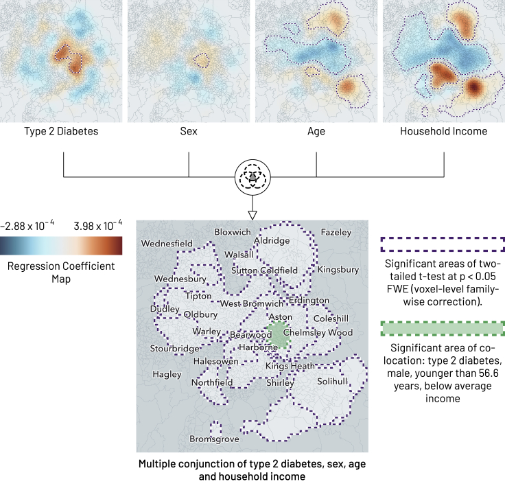
The characteristics and determinants of health and disease are often organized in space, reflecting our spatially extended nature. Understanding the influence of such factors requires models capable of capturing spatial relations. Drawing on statistical parametric mapping, a framework for topological inference well established in the realm of neuroimaging, we propose and validate an approach to the spatial analysis of diverse clinical data-GeoSPM-based on differential geometry and random field theory. We evaluate GeoSPM across an extensive array of synthetic simulations encompassing diverse spatial relationships, sampling, and corruption by noise, and demonstrate its application on large-scale data from UK Biobank. GeoSPM is readily interpretable, can be implemented with ease by non-specialists, enables flexible modeling of complex spatial relations, exhibits robustness to noise and under-sampling, offers principled criteria of statistical significance, and is through computational efficiency readily scalable to large datasets. We provide a complete, open-source software implementation.

Keywords: epidemiology; geostatistics; kriging; spatial analysis; statistical parametric mapping.

Figure 1

Sampling levels (noise-free, $\gamma =0.0$) for the univariate models on the left ($N=600,1200,1800$), and for the bivariate models on the right ($N=1600,3200$)

Figure 2

Example of a coverage computation for an instance of the bivariate snowflake model with noise $\gamma =0.1$ and $N=1600$ For each value $s$ of the smoothing parameter, the combined significant areas for all four spatial conditions $\left(Z_1,Z_2\right)\in \{(0,0),(1,0),(0,1),(1,1)\}$ as determined by a separate run of GeoSPM are shaded in light gray. The maximum number of significant grid cells is obtained for $s=40$, highlighted in red.

Figure 3

Synthetic snowflake models: recovery scores for GeoSPM and kriging of model term $Z_1$ in the low (N = 1600) and high (N = 3200) sampling regimes Lines denote the mean score across 10 random model realizations, shaded areas its SD to either side of the mean. Areas of overlapping performance are identified by additive shading. GeoSPM degrades more slowly and gracefully as noise increases compared with kriging. Comparable results for model term $Z_2$ are shown in Figure S10.

Figure 4

Synthetic anti-snowflake models: recovery scores for GeoSPM and kriging of model term $Z_1$ in the low (N = 1600) and high (N = 3200) sampling regime Lines denote the mean score across 10 random model realizations, shaded areas its SD to either side of the mean. Areas of overlapping performance are identified by additive shading. As is the case with the snowflake models, GeoSPM degrades more slowly and gracefully as noise increases compared with kriging. Comparable results for model term $Z_2$ are shown in Figure S11.

Figure 5

Recoveries of variable $Z_1$ in the synthetic bivariate snowflake model across $R$ = 10 repetitions for GeoSPM in the top row and kriging with a Matérn kernel and nugget component in the bottom row, both in the high sampling regime ($N$ = 3200) Grid cells that lie in the target region are shown in white, those outside in gray. The number of significant tests out of 10 repetitions is superimposed in color for each grid cell: dark blue indicates at least one significant test and dark red indicates the maximum number of 10, while cells with no significant test did not receive any color. Kriging only produces recoveries up to a $\gamma$ value of 0.10, whereas GeoSPM still produces recoveries for much higher values of $\gamma$. GeoSPM used t tests with a family-wise error corrected p value of 0.05, for kriging we applied a z-test with an uncorrected p value of 0.05, a null mean of 0.5 and a sample deviation obtained from the (positional) kriging variance estimate, as described in the section on “synthetic experiments: noise parameterization”. Additional kriging recoveries are shown in Figures S21–S25 of supplemental note S3.5.

Figure 6

Recoveries produced by GeoSPM for the synthetic interaction model across $R$ = 10 repetitions for variable $Z_1$ in the top row and term $Z_1\times Z_2$ in the bottom row, with N = 15,000 samples Grid cells that lie in the target region are shown in white, those outside in gray. The number of significant tests out of 10 repetitions is superimposed in color for each grid cell: dark blue indicates at least one significant test and dark red indicates the maximum number of 10, while cells with no significant test did not receive any color. Starting with a low value for the interaction effect $c_3$ on the left, recovery of the interaction term $Z_1\times Z_2$ in region $R_3$ is weak, while recovery for variable $Z_1$ in the same region is stronger. This correlates with the fact that observations $(1,1)$ occur with only a slightly elevated probability $p_3=0.6$ compared with their null probability of $0.525$ when $c_3$ equals $0$ in the same setting. As $c_3$ increases toward the right, recovery in the same region for term $Z_1\times Z_2$ increases ($p_3=0.725$ at the right), while recovery for variable $Z_1$ decreases (probability $p_1=0.125$ at the right for observing $(1,0)$, which is half of what it would be if there was no interaction effect). GeoSPM used t tests with a family-wise error corrected p value of 0.05.

Figure 7

Synthetic snowflake interaction model: recovery scores for SPM model variable $Z_1$ and term $Z_1\times Z_2$ with N = 15,000 samples Lines denote the mean score across 10 random model realizations, shaded areas its SD to either side of the mean. We increase the approximate interaction effect in region $R_3$ of the grid from left to right, so that the probability of observing $(1,1)$ grows while the probability of observing $(1,0)$ or $(0,1)$ shrinks (the probability of observing $(0,0)$ stays the same). As a result, scores increase for the interaction term $Z_1\times Z_2$ as it captures more of the overall variance, whereas scores for variable $Z_1$ decrease, until the only significant recovery occurs in region $R_1$, which represents half of the target for $Z_1$ and explains why the overall decrease saturates.

Figure 8

GeoSPM results for the four UK Biobank models of Birmingham (one column per model) Geographic regression coefficient maps are shown with outlines of significant areas in the corresponding two-tailed t test at p < 0.05 FWE (voxel-level family-wise correction). The smoothing parameter value is 7,000 m.

Figure 9

Geographic regression coefficient maps with location names for a single run of UK Biobank models 1 and 4 Model 1 is a univariate model of diabetes, model 4 adds sex, age, BMI, household income, and an interaction term BMI × household income. Outlines show significant areas in the corresponding two-tailed t test at p < 0.05 FWE (voxel-level family-wise correction). The smoothing parameter value is 7,000 m. The color map scale is the same as in Figure 8.

Figure 10

Binary conjunctions of geographic regression significance maps for a single run of UK Biobank model 4 A binary conjunction is formed of the significant areas of a two-tailed t test at p < 0.05 FWE (voxel-level family-wise correction) between type 2 diabetes and, in turn, sex, age, BMI, household income, and BMI $\times$ household income. Purple outlines show significant areas in the two-tailed t test of each variable, green outlines show significant areas of conjunction: significant areas of conjunction arise in diabetes combined with each of sex (male), age (younger than 56.6 years), BMI (below 27.9 kg/m²), and household income (below £35,015). No significant areas of conjunction exist for diabetes and BMI $\times$ household income. Locations shown in darker gray tone are not significant for any of the variables. The smoothing parameter value is 7,000 m.

Figure 11

Example of a multiple conjunction (here quaternary) of geographic regression significance maps for a single run of UK Biobank model 4 A binary conjunction is formed of the significant areas of a two-tailed t test at p < 0.05 FWE (voxel-level family-wise correction) between type 2 diabetes and, in turn, sex, age, BMI, household income, and BMI $\times$ household income. Purple outlines show significant areas in the two-tailed t test of each variable, green outlines show significant areas of conjunction: we can identify a significant area where younger males of lower income are associated with having type 2 diabetes in Birmingham. The smoothing parameter value is 7,000 m.

References

1. Anselin L. Local indicators of spatial association—LISA. Geogr. Anal. 1995;27:93–115. doi: 10.1111/j.1538-4632.1995.tb00338.x. - DOI
1. Kulldorff M. A spatial scan statistic. Commun. Stat. Theory. 1997;26:1481–1496. doi: 10.1080/03610929708831995. - DOI
1. Shepard D. Proceedings of the 1968 23rd ACM National Conference. 1968. A two-dimensional interpolation function for irregularly-spaced data; pp. 517–524. - DOI
1. Rosenblatt M. Remarks on some nonparametric estimates of a density function. Ann. Math. Stat. 1956;27:832–837. doi: 10.1214/aoms/1177728190. - DOI
1. Wand M.P., Jones M.C. CRC Press; 1994. Kernel Smoothing. - DOI
LinkOut - more resources