The molecular structure of IFT-A and IFT-B in anterograde intraflagellar transport trains

Abstract

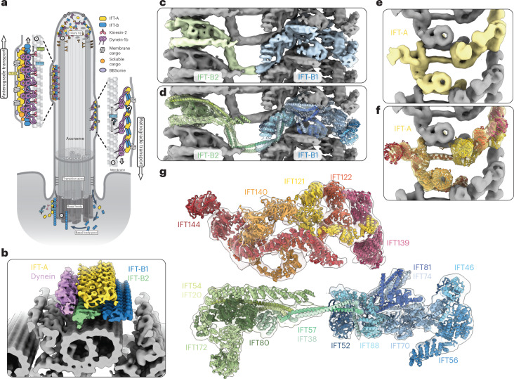
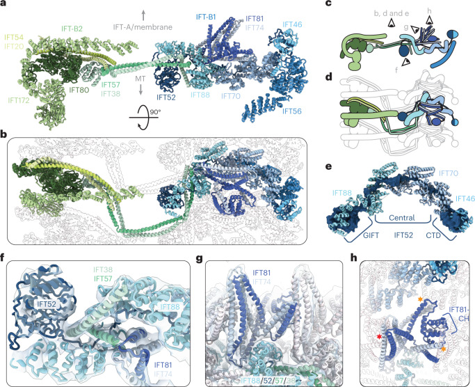
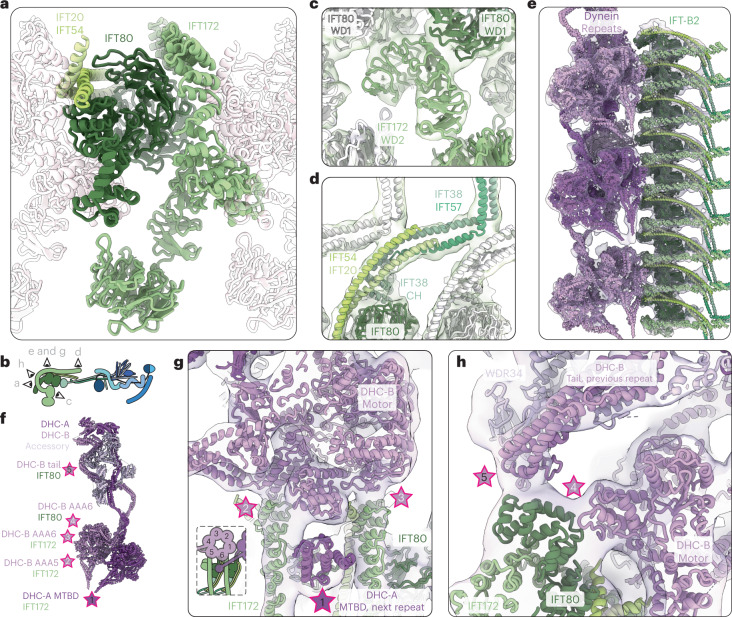
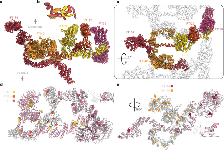
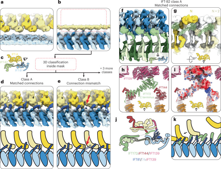
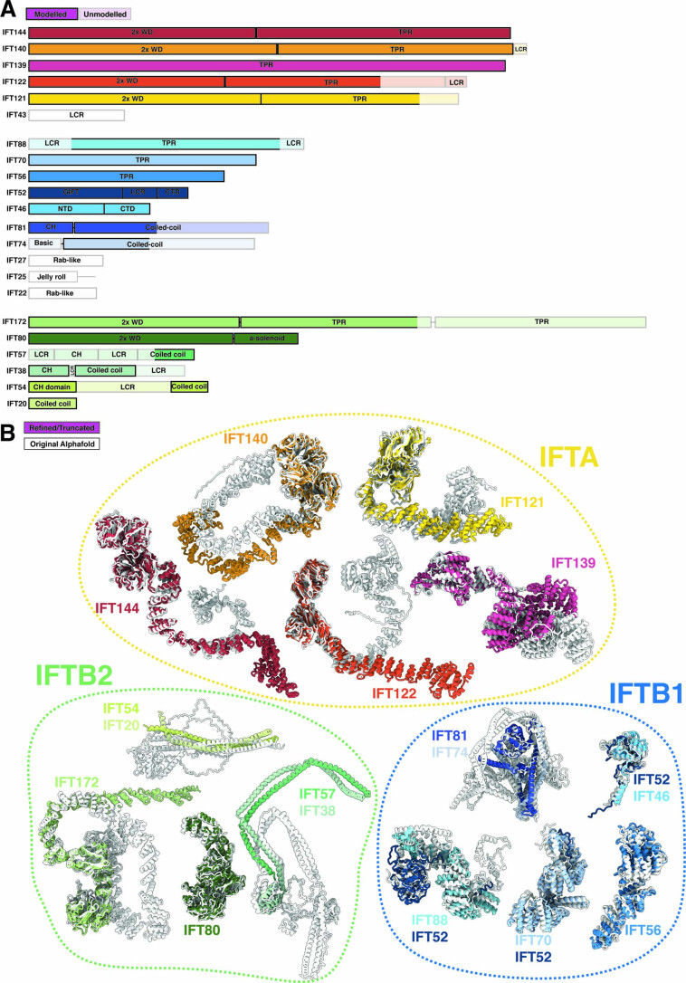
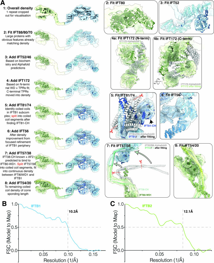
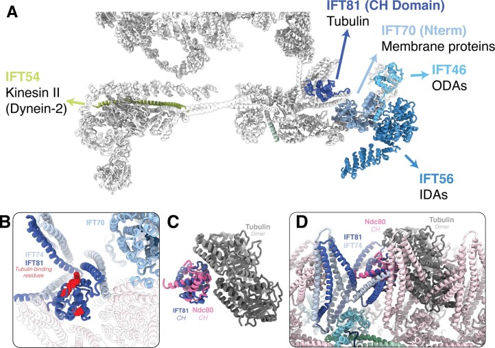
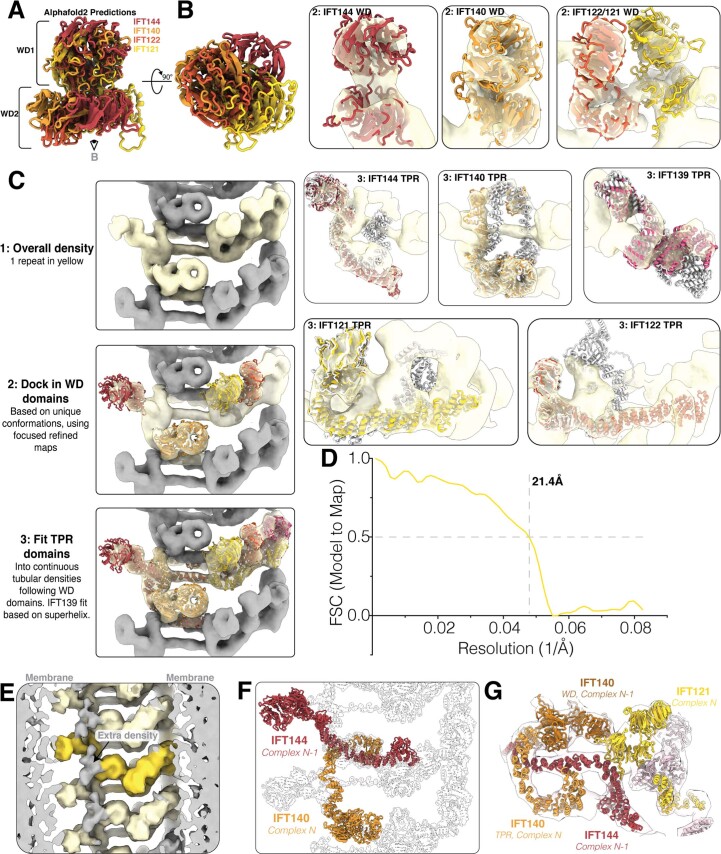
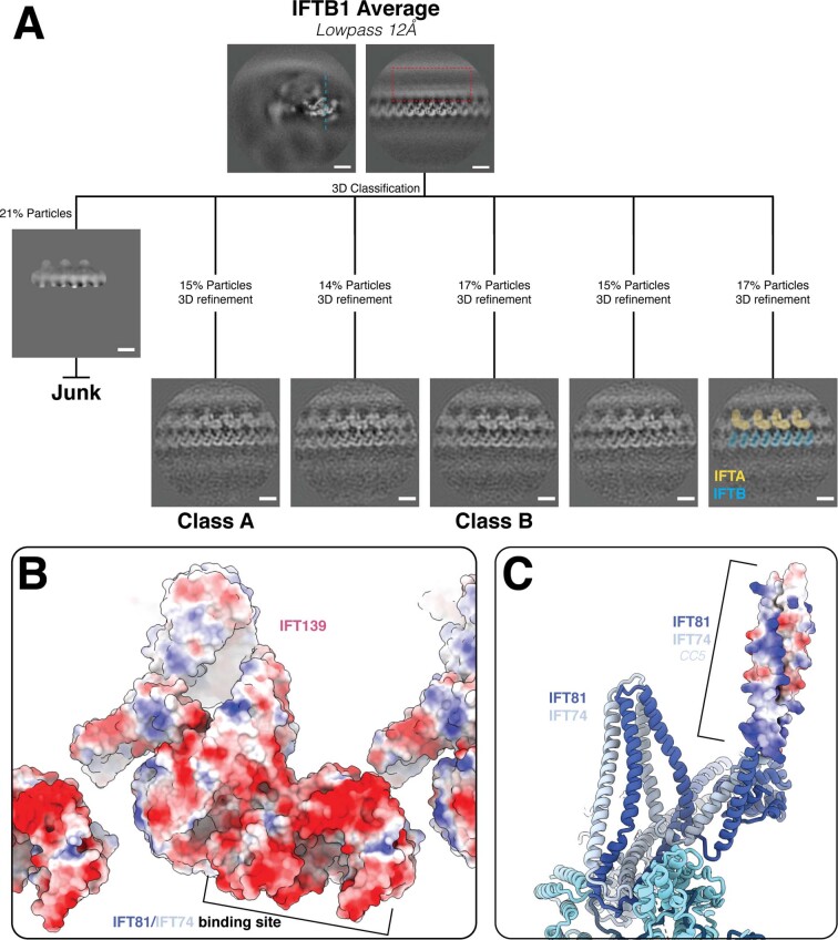
Anterograde intraflagellar transport (IFT) trains are essential for cilia assembly and maintenance. These trains are formed of 22 IFT-A and IFT-B proteins that link structural and signaling cargos to microtubule motors for import into cilia. It remains unknown how the IFT-A/-B proteins are arranged into complexes and how these complexes polymerize into functional trains. Here we use in situ cryo-electron tomography of Chlamydomonas reinhardtii cilia and AlphaFold2 protein structure predictions to generate a molecular model of the entire anterograde train. We show how the conformations of both IFT-A and IFT-B are dependent on lateral interactions with neighboring repeats, suggesting that polymerization is required to cooperatively stabilize the complexes. Following three-dimensional classification, we reveal how IFT-B extends two flexible tethers to maintain a connection with IFT-A that can withstand the mechanical stresses present in actively beating cilia. Overall, our findings provide a framework for understanding the fundamental processes that govern cilia assembly.

Fig. 1. An overview of the anterograde IFT train structure.

a, Cartoon model of IFT within a cilium. Anterograde trains form at the base of the cilium (basal body) and carry cargo through the diffusion barrier (transition zone) and to the tip. Here, they remodel into retrograde trains that carry their cargos back to the basal body for recycling. b, The new subtomogram averages lowpass filtered and colored by complex (yellow, IFT-A; blue, IFT-B1; green, IFT-B2; purple, dynein), docked onto a cryo-ET average of the microtubule doublets found in motile cilia. One repeating unit is highlighted in each complex with darker shading. c, The new subtomogram averages for IFT-B1 (blue) and IFT-B2 (green), displayed together as a composite. One repeating unit is highlighted in color, with the adjacent repeats in gray. d, Equivalent to c, but with the highlighted repeat now shown partially transparent and our molecular model of IFT-B docked in. e, The new subtomogram average of IFT-A, with one repeating unit shown in yellow and adjacent repeats in gray. f, Equivalent to e, but with the highlighted repeat now shown partially transparent and our molecular model of IFT-A docked in. g, Our molecular model of one repeating unit of IFT-A and IFT-B in the anterograde train, shown in cross-section as if looking down the microtubule. The partially transparent density for four maps is shown: IFT-B2 and IFT-A, with the main IFT-B1 average combined with a masked refinement of the region containing IFT56 (IFT-B1 tail; Extended Data Fig. 2a), since this region is more flexible relative to the core.

Fig. 2. IFT52 is central to the overall IFT-B complex.

a, One repeat of the IFT-B complex viewed in profile, looking down the train. MT, microtubule doublet. b, Top view of the IFT-B polymer, as if looking down from the membrane/IFT-A. A single repeat is shown in color, with adjacent repeats shown in silhouette. The coloring is as in a. c, Cartoon representation of a, showing the viewing positions of other panels in the figure. d, Cartoon representation of b. e, IFT52 (dark blue), shown as a molecular surface, forms the core of the IFT-B1 complex, with the central unstructured domain threading through the TPR superhelices of IFT88 (cyan) and IFT70 (steel blue). f, IFT57/38 (dark and light green, respectively) from IFT-B2 interact with IFT-B1 by fitting into a cleft in the TPR superhelix of IFT88 (cyan) along with the unstructured IFT52 central domain (dark blue). g, IFT81/74 (navy blue and gray, respectively) sit on top of IFT88 and form a compressed segmented coiled coil repeating along the IFT train. h, Top view of g. Lateral interactions with IFT81/74 in adjacent repeats are highlighted with stars (red star, IFT81-CH on N − 1 repeat; orange stars, IFT81/74-CC and IFT70 of N + 1 repeat).

Fig. 3. Interaction between IFT-B2 and dynein-2.

a, IFT80 (dark green) forms the core of the IFT-B2 complex. It is surrounded by IFT172 (olive green) and the IFT54/20 (lime green and pale green, respectively) coiled coil. Adjacent repeats are shown in silhouette. b, Cartoon representation of IFT-B depicting the positions of the views in the other panels. c, The second WD domain of IFT172 (olive green) does not close into a ring, and bridges two IFT80 subunits (dark green from the same complex and white in the neighbor). d, In the center of the complex, IFT54/20 (lime and pale green, respectively) and IFT57/38 (turquoise and mint green, respectively) coiled coils stack on top of each other, stabilizing a kink in IFT57/38 to point the subsequent coiled coils toward IFT-B1. e, The flexibly refined dynein models (purple and pink) docked into the 16 Å dynein density, along with the IFT-B2 model. f, Cartoon representation of cytoplasmic dynein-2 refined into our density, with the points that contact IFT-B2 and the protein they interact with highlighted with stars. g, Top view of the train, showing the first three contact points between dynein and IFT-B2. h, The two remaining contact points between dynein and the edge of IFT-B2, at the C terminus of IFT80.

Fig. 4. IFT-A presents its four WD domains to the membrane.

a, The IFT-A model viewed in profile, as if looking down the train. b, Cartoon representation of IFT-A shown from a side view as in a. c, Top view of the IFT-A model, with neighboring repeats shown as silhouettes. IFT140 and IFT144 both reach into the neighoring complex. d, We mapped alterations in human IFT-A proteins caused by point mutations that are linked to ciliopathies to conserved residues in C. reinhardtii. Here, IFT121, IFT122 and IFT139 are shown, with most alterations (shown as sphere representation) mapping to the WD domains or to interfaces between TPR domains. e, A second view, showing the alterations caused by point mutations present in IFT144 and IFT140.

Fig. 5. IFT-A and IFT-B are connected at two points.

a, The 21 Å IFT-A average covering three repeats, unmasked to show that IFT-B (light blue) is averaged out with respect to IFT-A (alternating yellow) due to peridocity mismatch. b, The IFT-B1 average filtered to 12 Å and unmasked, to show that IFT-A (yellow) is averaged out with respect to IFT-B1 (alternating blue) due to periodicity mismatch. The red box indicates the location of the mask used for subclassification to generate the classes in d and e. c, Cartoon depicting the view in a, b, d and e. d, After classification of the IFT-A region in the IFT-B1 average, we find classes where IFT-A (alternating yellow) and IFT-B (alternating blue) are in sync. We see a new density (dark blue) linking IFT-B to IFT-A, which we designate as CC5 of IFT81/74. Bottom, cartoon representation of the density. e, A second class shows how the IFT81/74 connections (dark blue) adapt to the periodicity mismatch between IFT-A (alternating yellow) and IFT-B (alternating blue), by switching register with respect to IFT-A at the red arrow. Bottom, cartoon representation of the density. f, A top view of class A from classification of the IFT-A region in the IFT-B2 average. Inset, cartoon view. IFT-B1 (alternating light/dark blue) and IFT-B2 (alternating light/dark green) are joined by a new, unmodeled density corresponding to the C terminus of IFT172 (lime green). g, The same class as f, rotated 180° to view the same IFT172 density (lime green and transparent, with the AlphaFold2 model docked) interacting with IFT-A. The IFT-A complex is colored to highlight that the connecting density connects nonadjacent neighbors. Inset, cartoon view. h, The same view as in g, showing the AlphaFold2 IFT172 C terminus model (lime green) docked into the density along with our IFT-A model. IFT172 bridges the gap between IFT144 and IFT139. i, The same view as in h, with IFT172, IFT144 and IFT139 shown with surface charge depiction. The negatively charged IFT172 C terminus can make favorable ionic interactions with the positively charged IFT144 C terminus. j, Cartoon representation of the overall anterograde train structure, showing the two points of connection (dotted outlines). k, Cartoon representation depicting the proposed role of the flexible tethers in recruiting IFT-A complexes to nascent IFT trains.

Extended Data Fig. 1. Identification of anterograde IFT trains in cryo-electron tomograms.

a, A slice through a representative tomogram from our dataset of a 600 tomograms of C. reinhardtii cilium, showing a bulge in the membrane in the middle corresponding to an anterograde IFT train (red box). Scale bar = 100 nm. b, Close up view of the train in A, with IFT-A (yellow) and IFT-B (blue) repeats annotated. Scale bar = 50 nm. c, After identification, we manually picked trains in IMOD as a contour running through the center of the complex. IFT-B picking is shown here, and IFT-A, visible above the IFT-B contour, was picked in a separate model. Scale bar= 50 nm. d, The contour was converted into subtomogram coordinates with oversampling to ensure no particles were missed. Scale bar= 50 nm. e, Here, the final refined coordinates are shown on the train. The particles have undergone proximity cleaning compared to the oversampling in D, as well as 3D classification to remove bad particles. Scale bar = 50 nm.

Extended Data Fig. 2. Processing diagram for IFT-B subtomogram averaging.

a, Workflow depicting the steps involved in averaging the IFT-B1 and IFT-B2 complexes. Processing started in STOPGAP (areas in dotted black line) before proceeding to Relion. The level of binning at each stage is indicated by the outline of the box (colour code top right). All scale bars=10 nm. b, The solvent masks used to refine IFT-B1 (blue) and IFT-B2 (green) separately from each other. c, The solvent masks used to refine the extremities of the IFT-B1 and IFT-B2 complexes, which are poorly resolved when using the masks in B. d,The solvent mask used to classify and refine dynein from IFT-B2. e, Fourier Shell Coefficient (FSC) curve of the IFT-B1 average, as a measure of map resolution. f, FSC curve of the IFT-B2 average.

Extended Data Fig. 3. Processing diagram for IFT-A subtomogram averaging.

a, Workflow depicting the steps involved in averaging the IFT-A complex. Processing started in STOPGAP (areas in dotted black line) before proceeding to Relion. The level of binning at each stage is indicated by the outline of the box (colour code top right). All scale bars=10 nm. b, The solvent mask used to refine IFT-A, containg one repeat. c, The solvent mask used to refine IFT-A, containing three repeats. d, The solvent mask used to refine IFT-A, consisting of the left side of one repeat of the complex. e, The solvent mask used to refine IFT-A, consisting of the right side of one repeat of the complex. f, Angular distribution of particles contributing to the IFT-A average (one repeat). g, FSC curve of the IFT-A average, refined using a mask containing one repeat. h, FSC curve of the IFT-A average, refined using a mask containing three repeats.

Extended Data Fig. 4. Alphafold2 models of IFT components.

a, Domain organization of all IFT constituents. Lighter shading indicates regions that were flexible and unmodelled in our structure. WD = WD40 repeat domain, TPR = Tetratricopeptide repeat domain, CH = Calponin homology domain, LCR = low-complexity (disordered) region. b, The original, unmodified alphafold structures (white) overlaid with the final refined models in our new structure (colours). Refined models have had flexible regions deleted.

Extended Data Fig. 5. Building a model of IFT-B using Alphafold2 predictions.

a, A step-by-step summary of the placement of each protein in IFT-B during molecular modelling, with accompanying illustrations shown in boxes on the right. 1: A single repeating unit of IFT-B cropped out of the overall composite map for visualization. IFT-B1 in blue and IFT-B2 in green. 2: We start by docking in unmodified Alphafold2 models of IFT88, IFT80 and IFT70, which have strong features and required few modifications to the Alphafold2 model 3: IFT52 was separately folded as a multimer with IFT88, IFT70 and IFT46 based on previous biochemical and structural data. The segments were joined back together and fit into the matching density. 4: IFT172 was initially identified through the strong fit between the density and the N-terminal WD-domains and TPRs in the Alphafold2 prediction (inset 4a), but the C-terminal TPR domains started to bend out of the density (inset 4b). We therefore moved the TPR domains into the continuous density emanating from the WD domains (arrow, inset 4b). 5: We concluded that the segmented coiled coil density on the top of IFTB1 was IFT81/74 based on previous studies. To fit the segments, we split them at the interconnecting loops (red scissor, as well as one more not shown in this view), fit them independently and then reconnected them. 6: IFT56 was docked in unchanged to the focused refinement of the periphery of IFTB1. 7: To place IFT57/38, we used the prior knowledge that IFT38-CH forms a high-affinity interaction with IFT80-WD1, and that IFT57/38 forms the link between IFT-B1 and IFT-B2. The linking density between the two lobes is a segmented coiled coil, matching the Alphafold2 prediction of IFT57/38. We therefore placed IFT38-CH in the small globular density bound to the face of IFT80-WD1, and split and docked the coiled coil segments into the bridging density. 8: IFT54/20 was the remaining Alphafold2 model to fit, and was docked into the coiled coil density of corresponding length in IFT-B2, the only region of the map left unmodelled. b,c, Model-to-map FSC curves for the IFT-B1 model into the IFT-B1 density and IFT-B2 model to IFT-B2 density respectively.

Extended Data Fig. 6. Building a model of IFT-B1.

a, A view of the IFT-B1 model docked into its density from the bottom (see E). b, A view of the IFT-B1 model docked into its density from the top (see E). c, Cartoon representation of IFT-B showing the views in A-D. d, A side view of the ‘tail’ of IFT-B1 docked into the masked tail refinement (Extended data 2A) map lowpass filtered to 18 Å. The region containing IFT56 was more flexible in the high-resolution average shown in A/B, but is more clearly resolved here. e, A close up view of IFT56 in the masked tail refinement map, showing that the twist in the TPR helix is visible. f, Density for the central unstructured domain of IFT52 (dark blue) is visible in the central pore of IFT88 (cyan), showing that the Alphafold2 prediction agrees with our experimental data. g, The N-terminal CH domain of IFT37 (light green) docks to the exterior face of the first WD domain of IFT80 (dark green) in IFT-B2. h, A proline residue (magenta) creates a kink in each of the IFT57/38 (dark/light green) helices near the contact to the first IFT88. i, The position of D268 in IFT52 highlighted in red, at the interface between IFT-B1 and IFT-B2. D268 in C. reinhardtii corresponds to the D259H mutation in humans.

Extended Data Fig. 7. Building a model of the IFT-B2 complex and its interaction partner dynein-2.

a, A top view of the IFT-B2 subtomogram average density with the IFT-B2 model docked in. b, A view of the end of the IFT-B2 subtomogram average density with the IFT-B2 model docked in. c, The same view as B, but at a lower threshold to demonstrate that IFT172-WD1 is represented in the density but at lower resolution than the rest of the complex due to flexibility. d, Cartoon depicting the views of IFT-B in the other panels. e, The IFT172-WD1 domain folded as a multimer with the CH domain of IFT57 forming a complex that is represented in the density of the IFT172 masked refinement map. f, The IFT54/20 (lime/pale green) bridge the gap in the IFT80-WD2 ring. g, Coloured density of Fig. 3d, showing our newly refined dynein average. Dynein repeats are alternating pink/purple, IFT-B2 is green. h, Side view of F. i, Same view as G, with density made translucent and the models docked in. j, The density in our new dynein average cropped out around the original dynein model (white) shows that the heavy chain undergoes a rearrangement in our newly refined model (purple), leaving an unmodelled density (inset). k, The unmodelled density likely corresponds to a Tctex1 dimer (green), linking the motor domains to the tail. l, A view of the top surface of IFT-B2, corresponding to the site where the dynein MTBD binds. m, The same view with surface charge representations shown, highlighting a positively charged patch where dynein binds.

Extended Data Fig. 8. Cargo interactions in anterograde IFT trains.

a, The IFT-A and IFT-B models are displayed in grey, with regions of IFT-B previously linked biochemically to cargo transport labelled coloured. The large structural cargo interactions mostly occur at the edge of IFT-B1. IFT54 is thought to recruit kinesin II to anterograde trains, but this is not visible in our structure, probably due to flexibility. b, The CH domain of IFT81 (navy blue), with positive residues thought to be important for tubulin binding shown in red. Only a narrow space exists between the coiled coil domains of IFT81/74 nearby. c, Comparison between IFT81 CH domain (navy blue) and the CH domain of Ndc80 (pink) bound to microtubules (grey, PDB 3IZO), indicating strong structural homology between the two CH domains. d, The Ndc80:MT complex structure docked with the Ndc80-CH domain aligned to the IFT81-CH domain, simulating a potential interaction with tubulin cargo. Strong steric clashes occur between tubulin and IFT81/74 in the neighbouring repeat.

Extended Data Fig. 9. The IFT-A polymer is built around four tandem WD domain proteins.

a, A comparison between the four tandem WD domains found in IFT-A, aligned at WD1. WD2 adopts a unique conformation relative to WD in each of the four proteins (with the TPR domain emerging at different places), allowing us to dock the models into the density. b, Equivalent to A, but with 90° rotation to provide a bottom view of the WD2 domains. c, A step-by-step guide of the model placements in IFT-A. 1: One repeat of IFT-A highlighted in yellow. 2: WD domains were docked into the density according to the angle between WD1 and WD2, and the exit of the TPR domain from WD2. Focused refinements were used for this positioning (as shown in inset panels for 2). 3: TPR domains were fit into the continuous tubular densities emanating from each of the WD domains, with IFT139 identified as the remaining spiral density corresponding to the TPR superhelix. d, Model-to-map FSC curve for the IFTA model (into the overall 20.7 Å 3-repeat IFTA density). e, We lowpass filtered our IFT-A 3-repeat average, with regions containing part of our model coloured in yellow (dark yellow highlighting a single repeat). We see an extra density (grey) forming a bridge between the WD domains of IFT144 and IFT140 that is not formed by a protein in our model. f, Long distance interconnectivity between IFT144 and IFT140 from neighbouring complexes. The TPR domain of IFT140 (orange) reaches into the neighbouring complex and stabilize its copy of IFT144-TPR (dark red). g, Side view of F, with some extra subunits coloured and density shown. The TPR domain of IFT140 from the adjacent repeat stabilizes the conformation of IFT144. The WD domain of IFT140 (dark orange) sits on top of IFT144-TPR (both complex-1), meaning IFT140-TPR from complex 2 is determining the conformation of its neighbour. This stabilizes the binding site for IFT121-WD (yellow, complex 1).

Extended Data Fig. 10. Classification of synchronous IFT-A and IFT-B averages.

a, Processing workflow of the classification of the IFT-B average to generate the classes in Fig. 5 that show synchronous IFT-A and IFT-B. Scale bars = 10 nm. b, Surface charge representation of IFT139 shows that the IFT81/74 binding site is strongly negatively charged. c, Surface charge representation of IFT81/74 CC5 shows that it is positively charged, facilitating its interaction with IFT139.

References

1. Anvarian Z, Mykytyn K, Mukhopadhyay S, Pedersen LB, Christensen ST. Cellular signalling by primary cilia in development, organ function and disease. Nat. Rev. Nephrol. 2019;15:199–219. doi: 10.1038/s41581-019-0116-9. - DOI - PMC - PubMed
1. Reiter JF, Leroux MR. Genes and molecular pathways underpinning ciliopathies. Nat. Rev. Mol. Cell Biol. 2017;18:533–547. doi: 10.1038/nrm.2017.60. - DOI - PMC - PubMed
1. Van den Hoek H, et al. In situ architecture of the ciliary base reveals the stepwise assembly of intraflagellar transport trains. Science. 2022;377:543–548. doi: 10.1126/science.abm6704. - DOI - PubMed
1. Dai J, Barbieri F, Mitchell DR, Lechtreck KF. In vivo analysis of outer arm dynein transport reveals cargo-specific intraflagellar transport properties. Mol. Biol. Cell. 2018;29:2553–2565. doi: 10.1091/mbc.E18-05-0291. - DOI - PMC - PubMed
1. Liu P, Lechtreck KF. The Bardet–Biedl syndrome protein complex is an adapter expanding the cargo range of intraflagellar transport trains for ciliary export. Proc. Natl Acad. Sci. USA. 2018;115:E934–E943. - PMC - PubMed
Publication types