Integrated intracellular organization and its variations in human iPS cells

Abstract

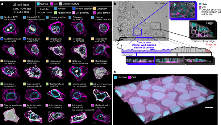
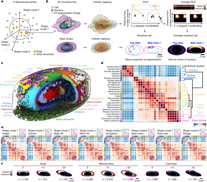
Understanding how a subset of expressed genes dictates cellular phenotype is a considerable challenge owing to the large numbers of molecules involved, their combinatorics and the plethora of cellular behaviours that they determine^1,2. Here we reduced this complexity by focusing on cellular organization-a key readout and driver of cell behaviour^3,4-at the level of major cellular structures that represent distinct organelles and functional machines, and generated the WTC-11 hiPSC Single-Cell Image Dataset v1, which contains more than 200,000 live cells in 3D, spanning 25 key cellular structures. The scale and quality of this dataset permitted the creation of a generalizable analysis framework to convert raw image data of cells and their structures into dimensionally reduced, quantitative measurements that can be interpreted by humans, and to facilitate data exploration. This framework embraces the vast cell-to-cell variability that is observed within a normal population, facilitates the integration of cell-by-cell structural data and allows quantitative analyses of distinct, separable aspects of organization within and across different cell populations. We found that the integrated intracellular organization of interphase cells was robust to the wide range of variation in cell shape in the population; that the average locations of some structures became polarized in cells at the edges of colonies while maintaining the 'wiring' of their interactions with other structures; and that, by contrast, changes in the location of structures during early mitotic reorganization were accompanied by changes in their wiring.

Fig. 1. The WTC-11 hiPSC Single-Cell Image Dataset v1 includes 25 cell lines that represent key cellular structures located throughout all of the major compartments of the cell.

a, Maximum intensity projections of one representative cell example per cellular structure, based on segmentations of the structure (white), the cell membrane (magenta) and the DNA (cyan). The fluorescently tagged protein representing the structure and the cellular compartment (Fig. 3d) are indicated. DFC, dense fibrillar component; ER, endoplasmic reticulum; GC, granular component. b, Top and side views (single slice) of hiPS cells with FP-tagged microtubules (via α-tubulin), grown in tightly packed, epithelial-like colonies and labelled with cell-membrane (magenta) and DNA (cyan) dyes to permit imaging and segmenting of cells and nuclei. Cells were most frequently imaged halfway towards the centres of large, well-packed colonies (blue) where they behave most consistently, but were also imaged at other locations within the colony, such as at the edges of colonies (red). z_lab denotes the lab frame of reference. c, Three-dimensional visualization of cell and DNA segmentations within a colony of hiPS cells. Total numbers of acquisition days, FOVs and cells per cellular structure are in Supplementary Data 1 and Extended Data Fig. 1d. Scale bars, 10 µm.

Fig. 2. A PCA-based cell and nuclear shape space reveals interpretable modes of hiPS cell-shape variation.

a, Segmented 3D images of a cell and its nucleus are rotated in the xy plane by θ_cell degrees around the cell centroid such that the longest axis of the cell is parallel to the x axis. These aligned images are the input for SHE of degree L_max = 16, resulting in a total of 578 SHE coefficients (289 for each the cell and the nucleus), which are used to reconstruct the cell and nuclear shape and nuclear location with high accuracy. x_lab, y_lab and z_lab denote the lab frame of reference and x_cell and y_cell the rotated cell frame of reference. Scale bar, 10 μm. b, Frequency of cells per map point bin (left) and explained variance (right) for the first eight principal components (PCs) of the PCA applied to the SHE coefficients for interphase cells (n = 202,847). Blue denotes one map point bin. c, Eight shape modes comprise the cell and nuclear shape space. Each is a normalized PC (standard deviation (s.d.), σ, units) sampled at nine map points (−2σ to 2σ in steps of 0.5σ). Three-dimensional shape reconstructions can be created at each of these map points—here yellow dots at the origin (0,0,0,0,0,0,0,0)—using an inverse PCA transform and its resultant SHE coefficients. Three 2D views of the 3D shape are shown. d, Most relevant 2D view of 3D shapes reconstructed at each of the nine map points for each of the eight shape modes (given names that can be interpreted by humans). Supplementary Video 1 shows all three 2D views. The centre bin in all modes is the identical mean cell shape. e, Overlay of 2D views of the cell (magenta) and nucleus (cyan) for the two most extreme map points (at −2σ, lighter, and 2σ, darker) of each shape mode. Source data

Fig. 3. Creating an average pairwise spatial interaction map of cellular structures.

a, Diagram illustrating the clustering of the 35,633 cells closest to the origin of an 8-dimensional sphere centred at the origin of the shape space. b, Creating average morphed cells. Top left, 3D visualization of the segmentations of a cell (magenta), nucleus (cyan), and cellular structure (here Golgi in white). Bottom left, the equivalent for the mean cell and nuclear shape. ‘Cellular mapping’ shows the results of interpolating the SHE coefficients to generate successive 3D concentric mesh shells (different colours) from the centroid of the nucleus (black dot) to the nuclear (inner) and then to the cell (outer) boundary to create the nuclear and cytoplasmic mapping, respectively. The presence or absence of the structure is recorded at each mesh point location, resulting in a PILR, shown in matrix format for the Golgi of this cell. The PILR of an individual cell or the ‘average PILR’ of the 1,058 Golgi-tagged cells within the 8-dimensional sphere can be mapped into the mean cell and nuclear shape, generating ‘morphed’ and ‘average morphed’ cells, respectively. Scale bars, 5 μm. c, Integrated 3D visualization of 17 of the 25 structures to illustrate their average relative spatial relationships (Supplementary Video 2). d, Average pairwise spatial interaction map of cellular structures. Heat map of the average location similarities (Pearson correlations between average PILRs; Extended Data Fig. 4g) for every pair of 25 cellular structures for cells in the 8-dimensional sphere. A clustering algorithm generates the dendrogram (left) with coloured branches of the six top-level clusters lengths representing the distance between clusters. e, Average spatial interactions are robust to systematic variations in cell and nuclear shape. Heat maps for the −2σ (bottom triangle) and 2σ (top triangle) shape space map points for each of the eight shape modes (numbers of cells and heat map data in Supplementary Data 1). f, Side view 1 of average morphed cells for three structures and three bins (0, −1 and −2σ) along shape mode 3 (major tilt). Scale bars, 5 μm. Source data

Fig. 4. Cellular structure locations are polarized but cellular structure location wiring is unaltered in cells at the edge of hiPS cell colonies.

a, Alignment. Cells at the edge of the colony are rotated in xy so that the axis between the cell centroid and the external contour midpoint is parallel to the x axis and the outer contour edge of the cell is oriented to the right. b, Mean cell (magenta or purple) and nuclear (cyan or green) shape for all interphase cells (left), edge cells (centre) and the shape-matched non-edge cells and edge cells combined. Three 2D views of the 3D shape are shown. Scale bar, 5 μm. c, Frequency of cells for the eight shape modes (SM) for all interphase (grey), non-edge (black) and edge (red) cells. d, Average morphed cells for mitochondria in non-edge and edge cells. e, ALP via LDA. PILR-LDA-based reconstructions of mitochondria in average morphed cells at five positions (in σ units) along the LDA axis. Dotted lines correspond to the locations of the mean non-edge (black) and edge (red) cells in d. f, Frequency of cells along the LDA axis within non-edge and edge cell populations. Dotted vertical lines indicate the means. g, Top view and side view 1 of three examples of non-edge and edge cells along the LDA axis. Top row shows the original and bottom row the morphed visualizations for each of these cells. Images are average projections of the segmented structure. h, The ALP for 25 cellular structures in edge cells. i,j, Heat maps of the average location similarity (i), stereotypy (j, left) and concordance (j, right) in non-edge cells (top triangle or left column in stereotypy) and edge cells (bottom triangle or right column in stereotypy). Numbers of cells and heat map data are in Supplementary Data 1. Scale bars, 5 μm. Source data

Fig. 5. Integrated intracellular reorganization in early mitosis.

a, Individual cell examples (top) and average morphed cells (bottom) for four cellular structures in prophase (m1) and early prometaphase (m2), shape matched to interphase cell subsets i1 and i2, respectively (Extended Data Fig. 10b). Cyan DNA outlines were left out for the histones and nuclear envelope to better see their locations at the nuclear periphery. Scale bars, 5 μm. b, The ALP and its timing of change (TOC) for 25 cellular structures in early mitosis. Asterisk indicates centriole ALP determined by visual inspection (Supplementary Methods). c, Left, heat maps of stereotypy (blue to red) and stereotypy differences (green to purple) in early mitosis. Black dots indicate values below the measurable cut-offs (Methods). Right, flagged significant stereotypy differences for each structure between interphase and both early mitotic stages (filled black boxes) as well as the resultant stereotypy TOC. The stereotypy of the plasma membrane was so high that, although the absolute difference in stereotypy values passed the flag criteria, the relative values were extremely small (denoted with ‘x’). d, Timing and types of change in concordance, through the PILR average correlation matrix. Bottom triangle: the concordance TOC assignments for all pairs of structures. Heat maps of intermediate steps are in Extended Data Fig. 10d–g and Supplementary Data 1. Top triangle: types of changes in concordance relative to changes in stereotypy as described in the results (Methods). Numbers range from n = 6 to 256 cells depending on the structure and stage (Supplementary Data 1). Coloured bars at the left of heat or colour maps in b–d indicate the cellular structure. Owing to the low number of cells in mitosis for some structures, we could not quantitatively analyse differences in the average location similarities, although their qualitative results matched those based on the concordance values (Extended Data Fig. 10g). e, Summary of examples of changes in distinct aspects of organization observed throughout this study. Specific examples are indicated with numbers: (1) structures that maintained locations in edge cells and early mitosis; (2) structures that polarized in edge cells; (3) for example, histones and microtubules at m1; (4) for example, histones and microtubules at m2; (5) most structures during early mitosis. Source data

Extended Data Fig. 1. Creation of the WTC-11 hiPSC Single-Cell Image Dataset v1 that contains over 200,000 live, high-resolution, 3D cells spanning 25 cellular structures.

The dataset was generated by a microscopy pipeline composed of three main parts; Data Collection, Image Processing and Single-Cell Feature Extraction. a. Data Collection: the sample preparation starts with a vial of frozen gene-edited hiPS cells from a line from the Allen Cell Collection, expressing an endogenous, fluorescently tagged protein representing a particular cellular structure. The cells are cultured in 6-well plates on an automated cell-culture platform. At each passage cells are seeded into optical grade, glass-bottom 96-well plates to create imaging samples. Bright-field overview images of each well are inspected and only wells meeting pre-determined quality controls are passaged from the 6-well plates and imaged from the 96-well plates. The image acquisition of live cells starts with a 12X overview image of each well on a spinning-disk confocal microscope to keep track of the position of each image within each colony. Imaging sessions are conducted using three modes to capture variations in colony area, locations within the colony, and enrich for images with mitotic cells as needed. In mode A, the 12X overview images of colonies are segmented by an automated script to generate sets of coordinates for positions within imageable colonies, located approximately halfway between the colony edge and colony centre. Imageable colonies are those that meet size, morphology, and position-within-a-well criteria. In mode B, the microscope operator adjusts the location of the field of view (FOV) to enrich for mitotic cells via appropriate cell and DNA morphology visible with live bright-field viewing and confirmed by DNA staining (yellow arrows). In mode C, three regions of colonies are imaged, the edge, ridge (just inward from the edge), and centre. The combination of these three imaging modes permitted sampling across all regions of the hiPS cell colonies (Extended Data Fig. 12). Cells were labelled with fluorescent DNA and membrane dyes and then imaged at each pre-selected colony position. Z-stacks were acquired at 120X in four channels, representing the bright-field, cell-membrane dye (magenta), DNA dye (cyan) and the fluorescently tagged cellular structure (grayscale), also shown in (b). Mode A and C panels show Golgi (via sialyltransferase) and microtubules (via alpha-tubulin), respectively. b. Image Processing: The WTC-11 hiPSC Single-Cell Image Dataset v1 consists of a total of 18,100 FOVs curated specifically for successful cell and cellular structure segmentations, which are available for download. An example z-stack is shown. On the left is the maximum intensity projection of all 65 slices with all fluorescent channels combined, in the colours indicated in the panels on the right. “Cutting” the z-stack in half exposes the view of a single slice (slice 32) in the middle of the stack, shown for each individual channel, including the bright-field channel. We applied 3D segmentation algorithms to each of the fluorescent channels to identify boundaries in 3D of the cells via the membrane dye (magenta), the nuclei and mitotic DNA via the DNA dye (cyan), and each of the 25 cellular structures via their fluorescent protein tag (grayscale; Golgi shown here). Resulting 3D segmentations for cell membrane, DNA, and structure channels are also shown as a side view, the xz-cross-section along the yellow dotted line. All segmentation algorithms were developed and performed using the Allen Cell & Structure Segmenter. c. Single Cell Feature Extraction: A total of 215,081 single cells were segmented from the FOVs. Every individual cell was labelled with a unique ID and metadata related to the sample, experiment, and microscopy was collected and associated with each individual cell for future data provenance. Appropriate features were extracted for each cell from the cell, the nucleus or mitotic DNA, and the cellular structure segmentations, including measurements such as the height and volume. These cells, including the images and the segmentations as well as the metadata and features are all available for download. Scale bars are 10 µm unless otherwise noted. d. Number of cells for each cellular structure in the WTC-11 hiPSC Single-Cell Image Dataset v1, sorted by their acquisition order. This table includes all of the various different subsets of the data used throughout the study, including the baseline interphase dataset (excluding outliers, see Methods), mitotic cells, cells within the 8-dimensional sphere (Fig. 3), cells at the edges of colonies (Fig. 4) and cells in early stages of mitosis (m1 and m2, Fig. 5).

Extended Data Fig. 2. Overview of cell, nuclear and cellular structure segmentations and caveats.

a. Panels show a representative single z-slice of the FP-tagged protein (left) and the target segmentation (right), demonstrating the degree of accuracy of the structure segmentations used for analysis. Several of these segmentations have specific types of caveats (b–d and Methods) that may affect interpretation of downstream analyses. b. The limits of the cell boundary segmentation algorithm include potential errors for the very top slices of each cell. Desmosomes, which localize to the cell periphery at the top of the cell, demonstrate this caveat well. Four sequential z-slices (z = 42-48) moving upwards towards the top of the cell-membrane dye signal are shown. In z = 42, both the cell-membrane dye and the cell segmentation clearly identify the true cell boundary (yellow arrows) and in z = 48, the in-focus desmosomes also line up well along the true cell boundary. However, in z = 46, the cell-membrane dye indicates two possible cell boundaries due to the slanted nature of the top of this cell and the out of focus light spreading from slices above and below. The in-focus desmosomes identify the inner possible boundary as the true cell boundary (yellow arrows). However, the segmented cell boundary is incorrect (cyan arrows). In z = 44 the desmosomes are not yet in focus, thus the true cell boundary is likely somewhere between that determined in z = 42 and z = 46. This error is negligible for overall cell segmentation, but critical for the assignment of desmosome locations in the cell. In this example shown, desmosomes are not located directly at the segmented cell periphery but still close by, such that a measurement of the total volume of desmosomes in this cell is still appropriate. However, it is equally likely that desmosomes, or any other structure localizing to the upper cell periphery could be mis-assigned to a neighbouring cell. Thus these structures were not considered validated for cellular structure volume analyses (Methods). c. Structures localizing or partially localizing to a thin 3D surface, such as the cell or nuclear periphery, may suffer from non-uniform accuracy between the middle and the top/bottom of that structure due to the anisotropic resolution of the images. Seven sequential z-slices (left) and target segmentations (right) of nuclear pores on the nuclear surface demonstrate this caveat well. The density of segmented nuclear pores is greatest at z = 36 and declines as the imaging plane moves upward through the nucleus. Consistently accurate detection for nuclear pores at both the centre and the top of the nucleus was not possible due to this effect and would require further algorithm development. The segmentation accuracy was sufficient to identify the general location of nuclear pores in cells for the location-based analyses but not sufficient to be validated for use in the cellular structure volume analysis. This caveat was also observed for other structures localizing to the nuclear and cell periphery (Methods). d. The segmentation target for cohesins (via SMC-1A) is to detect the most contrasted locations of cohesins in nuclei. This segmentation works well for nuclei in most of interphase (see example in (a)). However, SMC-1A moves from the cytoplasm back into the nucleus after mitosis. The amount of tagged SMC-1A protein in the nucleus and thus its segmentation depends on how far into interphase a cell is. Three examples of tagged SMC-1A are shown (left panels) along with the target segmentations (right panels). For a cell in early interphase (far left) SMC-1A is both in the cytoplasm and nucleus, but at low levels such that the target segmentation is quite sparse. For a cell well into interphase (far right), the target segmentation is as in (a). In the centre is a nucleus with moderate levels of SMC-1A and thus fewer cohesin locations segmented. e. Demonstration of the cell membrane Training Assay concept. Top row: tagged cell-membrane channel (via CAAX; left) and cell-membrane dye channel (right) images as single slices near the centre of the z-stack. Second row: corresponding side views of the same z-stacks. Bottom row: CAAX-based segmentation (left) and filled version for the cell-membrane dye-based segmentation performed on the dye image after training via the cell membrane Training Assay (right). The cell membrane at the top of cells is often very dim in the dye images (yellow arrows) due to both the very thin nature of the top membrane and photobleaching during z-stack acquisition. However, the top of these same cells is much more visible in the tagged plasma membrane cell line (cyan arrows), permitting successful CAAX-based segmentations. We leveraged the information contained in the CAAX images by using the CAAX-based segmentation as the training target for a deep learning cell-membrane dye-based segmentation model. f. Demonstration of the DNA dye Training Assay concept. Top row: tagged nuclear envelope channel (via lamin B1; left) and DNA dye channel (right) images as a single slice near the centre of the z-stack. Second row: corresponding side views of the same z-stacks. Bottom row: lamin B1-based segmentation (left) and filled version for the DNA dye-based segmentation performed on the dye image after training via the DNA dye Training Assay (right). The top boundaries of nuclei are often very blurry in the DNA dye images (yellow arrows) due to the “filled” nature of how the DNA dye demarcates the nuclear boundary combined with the diffraction of light and lower axial resolution. However, the top boundaries of nuclei in these same cells are clearly identifiable in the tagged nuclear envelope cell line (cyan arrows), permitting accurate nuclear segmentations via lamin B1. We leveraged the image information in the lamin B1 images by using the filled lamin B1-based segmentation as the training target for a deep learning DNA dye-based segmentation model. Total numbers of acquisition days, FOVs, and cells per cellular structure are in Supplementary Data 1 and Extended Data Fig. 1d.Scale bars are 3 µm for a–d and 5 µm for e–f.

Extended Data Fig. 3. A PCA-based cell and nuclear shape space reveals interpretable modes of shape variation in hiPS cells (supporting figure).

a. Mean distance between points in the original 3D meshes of cell (top) and nucleus (bottom) to their corresponding closest points in the reconstructed meshes and vice versa as the number of coefficients in the SHE increases. Each grey line is one cell (left; n = 300 randomly selected samples) or nucleus (right; n = 300 randomly selected samples). Black lines represent the mean. The dashed vertical lines indicate the number of coefficients for SHE degree L_max = 16. b. Two examples of how nine map points for each of the eight shape modes are used as the input for an inverse PCA transform to obtain the corresponding SHE coefficients and their corresponding 3D reconstructions at these map points. Three 2D views of the 3D shape are shown as in Fig. 2c. The top view corresponds to an intersection between the 3D mesh of the cell and nucleus reconstructions and the xy plane. Side views 1 and 2 correspond to an intersection between the 3D meshes and the xz- or yz-planes, respectively. c. Pairwise correlations for cell volume, cell height, and shape modes. Each point represents a single cell (n = 202,847). Points are colour-coded based on an empirical density estimate. The grey line represents the best linear fit. The green curve represents the non-overlapping window average (y-axis) within 100 equally spaced bins (x axis). Only results for bins with more than 50 points are reported. Pearson correlation values are indicated in the upper triangle part of the figure (black for non-zero values). d. Bar graph plots of the total variance explained by each PC for the shape spaces obtained when only nuclear (e) and cell (f) SHE coefficients are used as input for the PCA dimensionality reduction described in Fig. 2. e–f. Most relevant 2D view of 3D shapes reconstructed at each of the nine map points of each of the eight shape modes (given human-interpretable names). The centre bin in all modes is the identical mean cell shape. At the far right is an overlay of 2D views of the nucleus (e) or cell (f) for the two most extreme map points (at −2σ, lighter shade and +2σ, darker shade) of each shape mode. Source data

Extended Data Fig. 4. Creating and comparing integrated average cells throughout the shape space via SHE coefficient-based parameterization and 3D morphing.

a. “3-channel original z-stack” (bottom left image), shows a 3D visualization of the original FP intensities of tagged mitochondria (grayscale) in a single cell and nucleus, visualized via cell-membrane dye (magenta) and DNA dye (cyan). Moving rightward along the bottom row are the steps to create the PILR of the mitochondria via the FP signal in this cell. “3D reconstruction” (second image) shows the SHE-based 3D reconstruction meshes of the segmentations of this cell and nucleus. Next, “cellular mapping” shows the result of interpolating the SHE coefficients to create a series of successive 3D concentric mesh shells (different colours) from the centroid of the nucleus (black dot) to the nuclear (inner) and then to the cell (outer) boundary to create the nuclear and cytoplasmic mapping, respectively. The intensity values in the FP channel are recorded at each mesh vertex location, resulting in the “PILR” that is shown in matrix format in the fourth image. “Voxelization” shows the result when this PILR is converted back into a 3D image, voxel by voxel, into the same reconstructed cell and nuclear shape. Because this internal mapping is discrete, the resultant reconstructed image will have gaps. At the top, “original FP image (left) is the original image and “nearest neighbour interpolation” (right) is the voxelized PILR, now with the gaps filled using nearest neighbour interpolation. Voxel-wise Pearson correlation in 3D is used to compare these original and reconstructed FP images. b. Example PILRs (in matrix format as in a) for one cell for each of five cellular structures. Top view and side view 1 are shown on the far left. Top and bottom PILR matrices for each structure are based on the original FP image (grayscale on black background) or the structure segmentations (binary on white background), respectively. c. The FP-image-based PILR takes all intensities in the image into account, including any FP-tagged protein not localized to the target structure that the protein represents. For example, FP-tagged paxillin localized to matrix adhesions at the bottom of the cell but also throughout the cytoplasm. Two images of multiple cells (cell membrane indicated by magenta lines) in an FOV with labelled matrix adhesions (via paxillin) at two z positions in the z-stack. Top left triangles in each image show the original FP image. Matrix adhesions are visible near the bottom of the cells (left) but considerable FP-tagged paxillin signal is visible both at the bottom and centre (right) of cells. However, the segmentation target defined for this cell line included only the high intensity regions representing the matrix adhesions near the bottom of the cells. Bottom right triangles in each image show the result of the matrix adhesion specific segmentation. Total numbers of acquisition days, FOVs, and cells for FP-tagged paxillin are in Supplementary Data 1 and Extended Data Fig. 1d. d. Using the structure segmentation-based PILR permits the creation of average morphed cells containing the locations of the cellular structures that each tagged protein represents. Average morphed cells representing matrix adhesions (top row) and mitochondria (bottom row) generated using either the original FP images (left column) or the target structure segmentations (right column) of cells within the 8-dimensional sphere morphed into the mean cell shape. The analyses in this paper focus on the structure segmentation-based PILRs; but conceptually the same approach could also be applied to the raw intensity images. e. Bar graphs of voxel-wise Pearson correlation between original intensity images of FP-tagged proteins (left) or of structure segmentations (right) and the images reconstructed from the PILR. Error bars represent ± one standard deviation around the mean (n = 32 cells per structure). Cells were selected from centre bin of Shape Mode 1. The correlation for cohesins (via segmentations) is indicated with a striped fill pattern. This structure has a significantly changing target structure segmentation depending on how much tagged cohesin has re-entered the nucleus after mitosis, causing the much lower correlation value (Extended Data Fig. 2d). f. Example cell from the top of (a) to show the original and PILR-based reconstructed image but here based on the structure segmentations. Numbered insets are zoomed in regions. Cell and nuclear boundaries in a–f are shown in magenta and cyan lines, respectively. g. Overview of the process to calculate the average location similarity between all pairwise-combinations of the 25 cellular structures within the 8-dimensional shape space sphere. The 2D pixel-wise Pearson correlation was calculated between pairs of averaged PILRs for each structure. This created a correlation matrix including each of the 25 cellular structures with elements of this matrix representing the average location similarity between two cellular structures. h. Heat maps for the −2σ and 2σ shape space map points for each of the eight shape modes as in Fig. 3e, but here heat map values correspond to the difference in average structure similarity between the mean cell shape and either, the −2σ and 2σ shape space map points (bottom and top triangles, respectively), for each of the eight shape modes (numbers of cells in Supplementary Data 1). Due to technical considerations related to the PILR construction (Methods) or due to especially low number of cells in some bins (Supplementary Data 1), some structures displayed changes in the magnitude of the average location similarity with other structures in the shape mode bins furthest from the mean (−2σ and 2σ, mainly for Shape Mode 1) and so these decreases may not be biologically meaningful. Additional difference heat maps for intermediate shape mode bins are available in Supplementary Data  1. Source data

Extended Data Fig. 5. Overview panel for creating aggregated morphed cells for all 25 cellular structures.

a. Each row represents one of the 25 cellular structures (indicated by the colour bar on the far left). From left to right, on the left side of the large arrow, the first three sets of three images each show top view and side view 1 of three examples of individual cells with shapes similar to the mean cell shape (origin of the 8-dimensional sphere). For each set of three images, the left is the maximum intensity projection (MIP) of the original FP image (grayscale on black background), the centre is the average intensity projection of the structure segmentation image (AIP; binary on white background), and the right is the AIP for the structure segmentation-based PILR for that cell morphed into the mean cell shape. For nuclear envelope and nuclear pores, the centre slice, through the centre of the nucleus, of the original FP image is shown instead of the MIP. For these two structures and for histones, the cyan DNA outline has been left out to see the location of these structures at the nuclear periphery. b. On the right side of the large arrow are three different types of aggregations of the indicated number of individual morphed cells based on the structure segmentation PILRs. On the left is the average morphed cell, the centre is the standard deviation (std.) morphed cell, and the right is the “structure-localized coefficient of variation” (SLCV) morphed cell, representing a quantitative measure of how variable the location of a structure is at any given voxel (Supplementary Methods). Contrast settings for FP and AIP images were adjusted per cellular structure to best represent its location. Heat maps for average morphed cells indicate relative likelihood of a structure being at a given location in the cell. Heat map ranges for standard deviation morphed cell and SLCV morphed cell are as described (Supplementary Methods). Scale bars are 5 µm.

Extended Data Fig. 6. Location stereotypy and concordance are robust to systematic variation in cell and nuclear shape.

a. Heat map of the 2D pixel-wise Pearson correlation matrix for all pairs of cellular structure PILRs among all cells in the 8-dimensional sphere. Each entry in this matrix represents the correlation between the PILR of two cells. Coloured triangles to the left of, and the thicker black lines within, the matrix indicate the regions (blocks) of the matrix corresponding to cells with the indicated tagged structure. The dimensions of each block correspond to the number of cells. b. Average correlation matrix. Left: the location stereotypy for a cellular structure is the average of all the values in the blocks along the diagonal of the correlation matrix in (a). The numbers on the right indicate structures ranked by their stereotypy from greatest to least. Right: the location concordance for any two pairs of structures is the average of all the values in the corresponding structure pair block in the correlation matrix in (a). The diagonal of the concordance heat map corresponds to the stereotypy. Arrows indicate examples of the relationships between the heat maps in (a) and (b). c. Stereotypy heat maps for each of the eight shape modes (SM). Each row represents a different cellular structure and each column represent the nine binned map points along each shape mode (Fig. 2b). d. Concordance heat maps for the −2σ and 2σ shape space map points for each of the eight shape modes. The lower and upper triangles represent the −2σ and 2σ map points, respectively. Numbers of cells and heat map data in Supplementary Data  1. Colour bars on the left of heat maps indicate the cellular structure. Source data

Extended Data Fig. 7. Comparing location stereotypy and concordance throughout the cell and nuclear shape space.

a. Box plots of the diagonal values for each of the 25 cellular structures in the 3D voxel-wise Pearson correlation matrix heat map for all cells in the 8-dimensional sphere (Extended Data Fig. 6a). The thicker and shorter horizontal black line inside the box is the location stereotypy, the average of all the values in that structure’s block in the correlation matrix. Dots represent the raw data (one dot per correlation value; 1,000 randomly selected points are shown). The box extends from the first quartile (Q1) to the third quartile (Q3) of the data, with a line at the median. The whiskers extend from the box by 1.5x the interquartile range (IQR). Numbers of cells are in Supplementary Data  1. Colour bars along the bottom (x axis) indicate the cellular structure. Numbers above the colour bar indicate structures ranked by their stereotypy from greatest to least. The structures with the greatest location stereotypy were the nuclear envelope (lamin B1) and the plasma membrane (via CAAX domain of K-Ras, “CAAX”). These observations are effectively positive controls, because these two structures should be very similar to the cell and nuclear boundary shapes that were used as fixed points in the SHE interpolation. In decreasing order of stereotypy, the next highest were two nucleolar compartments, the Dense Fibrillar Component (DFC, via fibrillarin) and the Granular Component (GC, via nucleophosmin), followed by the ER (both Sec61 beta and SERCA) and microtubules. Structures with the least location stereotypy included those with a low number of discrete separated locations near the top or bottom of the cell such as centrioles (via centrin-2), desmosomes (desmoplakin), and matrix adhesions (paxillin) as well as structures with sparse, punctate locations such as cohesins (SMC-1A), endosomes (Rab-5A) and peroxisomes (PMP34). b. The process to create the Pearson correlation matrix for the 8-dimensional sphere (Extended Data Fig. 6a) was repeated for the reconstructed cell and nuclear shapes at each of the nine map points for each of the eight shape modes. Shown here are the resulting correlation matrices along Shape Mode 1. Each entry in this matrix represents the correlation between the cellular structure PILR of two cells. Thicker black lines within the matrix indicate the regions (blocks) of the matrix corresponding to cells with a tagged structure. The size of each dimension of each block corresponds to the number of cells. c. Heat maps of the difference in location stereotypy for each of the eight shape modes (SM). Each heat map represents a shape mode, each column represents the nine binned map points along that shape mode (Fig. 2b), and each row represents a different cellular structure. Each heat map value corresponds to the stereotypy difference between the mean cell shape and the cell shape in the indicated shape mode bin for that cellular structure. d. Heat maps of the difference in location concordance between the mean cell shape and either, the −2σ and 2σ shape space map points (bottom and top triangles, respectively), for each of the eight shape modes. Numbers of cells are in Supplementary Data 1. Colour bars on the left of heat maps indicate the cellular structure. Additional concordance difference heat maps are available in Supplementary Data 1. Source data

Extended Data Fig. 8. Statistical analysis of the variation in cell, nuclear and cellular structure sizes.

a. Heat map in four parts summarizing the results of a systematic, comparative analysis of the relationship between the volumes of the15 cellular structures validated for structural volume analysis and five cell and nuclear size metrics: the volume and surface area of the cell and the nucleus, and fifth, the cytoplasmic volume (the difference between cell and nuclear volumes), referred to as cell vol, cell area, nuc vol, nuc area, and cyto vol, respectively; Supplementary Methods). The number of cells in a–k are either all cells (n = 202,847) or per cellular structure (Extended Data Fig. 1d). The leftmost column (green heat map, scaling rate) indicates the percentage increase in structure volume given one doubling in cell volume over a well-represented volume range in the cell population (1160 to 2320 µm³). For example, the volume of mitochondria increased by an average 84% (from 108 to 199 µm³) for this doubling in cell volume (a doubling is an increase of 100%). The structures with the greatest relative scaling rates were the peroxisomes, followed closely by both nucleolar structures and then microtubules, all of which nearly doubled in structure volume with the doubling of cell volume. Simple linear regression was used to fit the data and to calculate the percent of the variation in cellular structure volumes that can be explained by each of the five cell and nuclear size metrics (next five columns in a, blue-red heat map, explained variance). The percent explained variance was substantially greater for some structures, such as mitochondria (54%) than for other structures, such as endosomes (2%). For nuclear structures like the nucleolar DFC, more of the variance in their volumes could be explained by nuclear volume than by cell volume (77% vs. 68%, respectively). A multivariate model was applied to calculate the total percentage of the variance explained for each of these structures by the combination of all four cell and nuclear size metrics (centre single column, all metrics). At the lowest end were the centrioles, which are discrete structures that double in number during the cell cycle, but with a negligible volume increase. Centrioles should not get continuously bigger as cells grow and were thus invariant with all size metrics. At the highest end were the nuclear envelope and the plasma membrane, which, as expected, correlated well with nuclear and cell surface areas, respectively. Notably, the volumes of all three nuclear body structures (nucleolar DFC, GC, and speckles) had high explained variances. Cell and nuclear metrics show a large degree of collinearity, which makes it non-trivial to isolate the effect of one particular cell or nuclear metric on structure volume. The multivariate model was used to calculate the unique contributions of both cell size metrics, both nuclear size metrics, and each of the four metrics individually (last six columns, orange heat map, unique explained variance). For all five nucleus-related structures, the variance in structure volume was better explained by nuclear size metrics than by cellular size metrics. For the nuclear envelope, more of the variance was uniquely attributable to the nuclear surface area than nuclear volume; this anticipated result confirmed the validity of this approach. b. Scatterplot of nuclear vs. cell volumes for all cells, coloured based on an empirical density estimate. The green line is a running average and the grey line is the linear regression model, also used to calculate the scaling rate (see a). c. Line plots showing the scaling rate for three cellular structures (yellow line and numbers in top left corners). The regions filled in grey are the interquartile range (IQR) measured across cells that were binned in 10 cell volume bins. The xy axes to the far left are used to indicate the values of the tick marks in each of the three plots. d–g. Scatterplots and statistical measures as in (b), for mitochondria (d), endosomes (e), and nucleoli (DFC, f and g). h. Scatterplot of the relative volume scaling rate vs. the total percent explained variance for the 15 cellular structures. Error bars are 5-95% confidence intervals calculated via bootstrap (n = 100). Structures along top and right side are rank ordered. The structures with the lowest relative volume scaling rates were also the structures identified as having the lowest explained variance (endosomes, centrioles). For most structures, however, relative scaling rates were at least 60%, consistent with the simple expectation that larger cells typically would also have larger organelles. Two structures whose volumes correlated most strongly with nuclear surface area (nuclear envelope, nuclear speckles) showed lower scaling rates. This was consistent with surface area generally scaling less quickly than volume. For example, doubling the size of a perfect sphere leads to only a 59% increase in its surface area. The peroxisomes stood out as exhibiting an unusual pattern of both a high relative volume scaling rate and great variability in peroxisome volume from cell to cell. i. Scatter plot of nuclear surface area vs. nuclear volume for all cells (blue points), cells with spherical nuclei (n = 19,927, brown points), perfect spheres (magenta dashed line) and linear and non-linear model fits on spherical cells or all cells (cyan and black as indicated; Supplementary Methods). The volume (V) and surface area (A) of a sphere don’t scale linearly, instead A ~ V^2/3. However, on this dataset a linear model of nuclear volume explains as much variation in nuclear area as a model with the theoretically correct non-linear scaling factor. j. Scatterplot of explained variance for linear vs non-linear models for all cases in the heat map of explained variance in a (n = 190; Supplementary Methods). Median (across 100 bootstraps of the regression model; blue points) and 95% confidence interval (from 2.5% to 97.5% across the 100 bootstraps; red lines) are indicated. k. Heat map of percent explained variance between size-scaling metrics (rows) and shape modes (SM, columns). Correlations of structure volume to Shape Mode 5 likely occur due the moderate correlation between Shape Mode 5 (elongation) and cell surface area. Source data

Extended Data Fig. 9. ALPs in shape-matched non-edge and edge cells.

a. Cell and nuclear SHE coefficients from a comparison dataset (e.g., edge cells; red dots) are transformed according to the SHE PCA of a baseline dataset (e.g. interphase cells; black + grey dots) resulting in the embedding of the comparison dataset cells into the baseline 8D shape space. Each cell in the comparison dataset is matched to its nearest neighbour in the shape space that is also in the baseline dataset (lines connecting black and red dots), creating the shape-matched dataset. b. Average morphed cells for six cellular structures in shape-matched non-edge and edge cells. For five of these structures, the ALP is a redistribution of the structure towards the outer edge of the colony, while for adherens junctions (via beta-catenin) the ALP is a redistribution of junctions away from the colony edge. c. Dimensionality of PILRs of cells in the shape-matched dataset is first reduced to 32 via PCA (see Methods). LDA is then applied to these 32 PCs to find the axis of greatest separation (solid purple line) between the two groups of cells in the dataset (black and red dots). Data points are projected along the discriminant axis to determine the frequency of cells. d. Average morphed cells for actin bundles (via alpha-actinin-1) in non-edge and edge cells. e. PILR-LDA based reconstructions of actin bundles in average morphed cells at five positions (in σ units) along the LDA axis. Dotted lines correspond to the locations of the mean non-edge (black) and edge (red) cells in (d). f. Frequency of cells along the LDA axis within non-edge and edge cell populations. Dotted vertical lines indicate the means. g. Top view and side view 1 of three examples of each non-edge and edge cells along the LDA axis. Top row shows the original and bottom row the morphed visualizations for each of these cells. Images are average projections of the segmented structure. h. Frequency of cells along the LDA axis within non-edge and edge cell populations for the five structures in (b). Dotted vertical lines indicate the means. PILR-LDA based reconstructions of average morphed cells at five positions (in σ units) along the LDA axis for all 25 cellular structures as well as single-cell examples available in Supplementary Video 3. i. Heat maps of the differences in average location similarity (left), stereotypy (centre) and concordance (right) for the 25 cellular structures in shape-matched non-edge vs. edge cells (numbers of cells and heat map data in Supplementary Data 1). Source data

Extended Data Fig. 10. Integrated intracellular reorganization in early mitosis (supporting figure).

a. We investigated two stages of early mitosis—prophase (m1) and early prometaphase (m2), when the condensing chromosomes still largely form an aggregated, nuclear-like structure that could be biologically interpreted in the context of our cell and nuclear shape-based coordinate system. Due to the breakdown of the nucleus and the condensation of DNA in these early stages of mitosis, the outline of the DNA-dye-based segmentation was no longer appropriate for SHE-based parameterization. Instead, we replaced the nuclear segmentation of cells in both datasets with their convex-hull counterpart. b. Mean cell (magenta or purple) and nuclear (cyan or green) shape for all interphase cells (1^st column), cells in prophase (m1), shape-matched interphase 1 and m1 cells (i1 + m1), cells in early prometaphase (m2), and shape-matched interphase 2 and m2 cells (i2 + m2), respectively. c. Frequency of cells for the eight shape modes (SM) for all interphase (grey), i1 (black) and m1 (red) cells (top two rows), i2 (black) and m2 (red) cells (bottom two rows). d. Concordance heat maps for interphase cells in the two shape-matched interphase datasets (i1, i2) and their corresponding prophase (m1) and early prometaphase (m2) mitotic cells. e. Heat maps of the differences in concordance in early mitosis for i1–i2, i1–m1, m1–m2, and i2–m2 stages. f. Flagged significant concordance differences (black boxes) for each of the difference heat maps shown in (e). g. Average structure similarity heat maps for interphase cells in the two shape-matched interphase datasets (i1, i2) and their corresponding prophase (m1) and early prometaphase (m2) mitotic cells. Due to the low number of cells in mitosis for some structures, we did not quantitatively analyse differences in the average location similarities, although their qualitative results matched those based on the concordance values. Heat maps in Supplementary Data 1. Source data

Extended Data Fig. 11. Summary of this study.

a. The Allen Cell Collection of high-quality gene-edited FP-tagged cell lines and the standardized microscopy imaging pipeline, combined with new tools for image analysis permitted us to create the WTC-11 hiPSC Single-Cell Image Dataset v1 of over 200,000 living cells and 25 cellular structures in 3D. b. We created two distinct conceptual coordinate systems to analyse our cells. The first maps the shape of an individual cell with respect to the total shape variation observed in the entire population via a 3D cell and nuclear shape space (via SHE). The second maps the location of every cellular structure within an individual cell (via the PILR). c. With these two coordinate systems we created an analysis framework to measure distinct aspects of integrated intracellular organization, including measurements of structure volume variations as well as the locations of cellular structures. This included the average locations both of individual structures and all pairs of structures (ALP and average structure similarities), as well as the variability in these locations (stereotypy and concordance). d. This suite of measurements was applied to our large baseline dataset of interphase cells and showed that integrated intracellular organization was very robust across the wide range of cell shapes in the normal interphase population. e. Two cell subpopulations stood out morphologically in the dataset: colony edge cells and mitotic cells, prompting us to assess their organization. To do this, we developed a process to match each individual cell in the chosen subpopulation with a “control” (interphase) cell of similar overall shape, and then used analysis of these shape-matched pairs to visualize and quantify the location phenotype of greatest difference between the two populations (via the PILR-LDA). f. First, we compared the intracellular organization of cells at the edges of hiPS cell colonies compared with shape-matched non-edge cells. We found that some structures showed a polarized location towards the colony edge but this change in location was not accompanied by any other changes in pairwise structure locations or variations, suggesting that while the locations changed, the variability and relationships among structures (average structure similarities, stereotypy, and concordance) i.e., the “wiring”, of the cell did not. g. In contrast, our second subpopulation comparison focused on early mitotic cells confirmed that they undergo a dramatic intracellular reorganization, in which not only the average locations of structures, but also their wiring, changed substantially. To assess these changes with a robust quantitative perspective, we developed new workflows to formally identify when significant changes in any of these measurements occurred in the first two early stages of mitosis, and then summarized and visualized these results in a way that could facilitate further data exploration and hypothesis generation. We found that all structures except those located at the cell periphery changed their average locations during early mitosis. Furthermore, all structures that changed location (other than the four for which stereotypy was statistically not measurable) also changed in at least one other aspect of their organization (stereotypy, concordance, or both) during at least one of the two stages of early mitosis. Thus, structure location changes of cells in early mitosis, unlike in edge cells, were accompanied by changes in their wiring. This suggests that edge cells and early mitotic cells may represent distinct classes of cellular reorganization, perhaps related to the specific cellular processes underlying them. h. We performed a meta-analysis to investigate the association between distinct aspects of cell organization observed throughout this study. The results of this meta-analysis prompted us to suggest a possible hierarchy of dependencies as cells reorganize, as outlined in the Discussion. However, our observations also demonstrate that this simple proposed hierarchy among these distinct aspects of organization is not absolute. It is possible that these potential dependencies, or “rules” of cell organization, are general and apply to a range of genetic perturbations, differentiation, signalling factors, environmental signals, etc. It is also possible that there is a larger set of cell type or state-dependent organizational rules.

Extended Data Fig. 12. Statistical analysis for quality control of the WTC-11 hiPSC Single-Cell Image Dataset v1.

a. Box plots of principal component values for all cell lines together (first bin in dark green) and per tagged structure cell line, plotted in pipeline timeline order, the order that structure datasets were collected (total n = 175,147; n per structure in Supplementary Data 1). The box extends from the first quartile (Q1) to the third quartile (Q3) of the data, with a line at the median. The whiskers extend from the box by 1.5x the interquartile range (IQR and dots represent outliers beyond the IQR. The dashed horizontal line spanning the entire plot represents the median value for all cell lines together (first bin in dark green). The colours for each cell line refer to the pipeline workflow (see Methods for details). Triangles indicated structures for which the IQR does not overlap with the mean value for all cell lines. b. Left plots shows the distributions of cell height (top) and cell volume (bottom) for all cell lines together (first bin in dark green; n = 202,847) and per tagged structure cell line, plotted in pipeline timeline order (n per structure in Supplementary Data 1 and Extended Data Fig. 1d). Structure names in red indicate those structures imaged with an adjusted Matrigel coating protocol towards the end of the pipeline timeline. The centre plots show a comparison of cell height (or volume, bottom) between actomyosin bundle-tagged cells (via non-muscle myosin IIB) in the main dataset (Pipeline 4.1; n = 6,223) and in a repeat dataset imaged with Pipeline 4.4 settings with the adjusted Matrigel coating protocol (n = 380). The right plots shows a comparison of cell height (or volume, bottom) between all cell lines imaged pre-Pipeline 4.4, during Pipeline 4.4 with original Matrigel coating and during Pipeline 4.4 with adjusted Matrigel coating. Percentages shown in the plot are the relative height reduction compared to the mean height of cell lines imaged pre-Pipeline 4.4. c. The top image diagrams circular mapping of imaged colonies (via the 12X overview images). Two cells are represented by two red dots within an FOV, represented by a rectangle. The FOV centre is at distance d from the closest edge of the colony. The two cells are then mapped into a unit circle that serves as a template to visualize the radial location of the two cells. The radial location is the FOV relative distance to the edge of the colony, ℓ = d/R_eff, where R_eff represents the effective radius of the colony. The angular location of a cell (θ₁ and θ₂ for the two cells in the image) is independently drawn from a uniform distribution of angles in the range [0,2π]. Cells from the dataset that were associated with a colony size (see Methods) were grouped into four bins, each with similar number of cells, based on the area of the colony where they came from. The colony area range of each bin is 15k-230k µm², 230k-377k µm², 377-620k µm² and 620k-14,285k µm². Each point represents one cell within the colony area bin that was mapped into the unit circle. The unit circle was then rescaled to match the mean colony area for that bin. Points are colour-coded by their corresponding cell height. Listed above each circle is the mean colony area in that bin to which the unit circle is scaled. Below each circle are profile plots of cell height as a function of the radial distance for each of the cell (in black). The red curve represents the rolling average. Each row of circular colony mappings represents a different aggregation of the data based on the imaging mode: the first row is for all imaging modes (modes A, B and C; n = 104,269), the second row is for modes A and B only (n = 75,146) and third row is for mode C only (n = 29,123). d. Circular colony mappings as in (c) where points (cells) are now colour-coded by values of the shape modes. Circular colony mappings are shown for Shape Modes 1 and 2, and profile plots (as in c), for Shape Modes 3-8 (all imaging modes, n = 104,269). e. Scatter plots on the far left show true values of cell height compared to cell height values predicted by random forest regression models (n = 95; see Methods) that include either all experimental variables (top plot) or all experimental variables except for the cell line identity (bottom plot). The error bars on the predicted values are obtained via bootstrapping (n = 100). The centre column shows box plots representing the feature importance for each of the two models as measured by the increase in the mean squared error (MSE) when all values of that corresponding feature are shuffled across samples. The box extends from the first quartile (Q1) to the third quartile (Q3) of the data, with a line at the median. The whiskers extend from the box by 1.5x the interquartile range (IQR and dots represent outliers beyond the IQR. The right top plot is the Pearson correlation matrix between five continuous experimental variables used in training the regression models. The bottom right plot is the Cramer’s V correlation matrix between six categorical experimental variables used in training the regression models. Variables with correlation above the significance threshold 0.3 are assumed to be highly correlated. Source data

References

1. Kirschner M, Gerhart J, Mitchison T. Molecular “vitalism”. Cell. 2000;100:79–88. doi: 10.1016/S0092-8674(00)81685-2. - DOI - PubMed
1. Woese CR. A new biology for a new century. Microbiol. Mol. Biol. Rev. 2004;68:173–186. doi: 10.1128/MMBR.68.2.173-186.2004. - DOI - PMC - PubMed
1. Karsenti E. Self-organization in cell biology: a brief history. Nat. Rev. Mol. Cell Biol. 2008;9:255–262. doi: 10.1038/nrm2357. - DOI - PubMed
1. Rafelski SM, Marshall WF. Building the cell: design principles of cellular architecture. Nat. Rev. Mol. Cell Biol. 2008;9:593–602. doi: 10.1038/nrm2460. - DOI - PubMed
1. Roggiani M, Goulian M. Oxygen-dependent cell-to-cell variability in the output of the Escherichia coli Tor phosphorelay. J. Bacteriol. 2015;197:1976–1987. doi: 10.1128/JB.00074-15. - DOI - PMC - PubMed
Publication types