Ensemble averaging: What can we learn from skewed feature distributions?

Abstract

Many studies have shown that observers can accurately estimate the average feature of a group of objects. However, the way the visual system relies on the information from each individual item is still under debate. Some models suggest some or all items sampled and averaged arithmetically. Another strategy implies "robust averaging," when middle elements gain greater weight than outliers. One version of a robust averaging model was recently suggested by Teng et al. (2021), who studied motion direction averaging in skewed feature distributions and found systematic biases toward their modes. They interpreted these biases as evidence for robust averaging and suggested a probabilistic weighting model based on minimization of the virtual loss function. In four experiments, we replicated systematic skew-related biases in another feature domain, namely, orientation averaging. Importantly, we show that the magnitude of the bias is not determined by the locations of the mean or mode alone, but is substantially defined by the shape of the whole feature distribution. We test a model that accounts for such distribution-dependent biases and robust averaging in a biologically plausible way. The model is based on well-established mechanisms of spatial pooling and population encoding of local features by neurons with large receptive fields. Both the loss functions model and the population coding model with a winner-take-all decoding rule accurately predicted the observed patterns, suggesting that the pooled population response model can be considered a neural implementation of the computational algorithms of information sampling and robust averaging in ensemble perception.

Figure 1.

A population coding model of ensemble perception. (A) The general architecture of the model. Here, an example set of few oriented lines (mean orientation 50°) is transformed into four individual orientation values (color circles) after corruption by a Gaussian early noise. Each value is represented as a component population response (dashed color distribution lines). The component responses are pooled by averaging to produce an ensemble representation (black solid line) with a peak location decoded as the average. (B) A histogram of an example stimulus orientation distribution: The count axis showing the number of items per feature value) with three shapes of hypothetical population responses to this distribution depending on the width of the tuning curve. The narrower the tunings, the more its peak (shown by a solid color line in each case) shifts away from the real mean (dashed vertical line) toward the mode. For illustration purposes, the population response curves are normalized by their peak activation.

Figure 2.

Stimuli and procedure of Experiments 1 and 2. (A) Orientation distributions from symmetric (mean–mode distance = 0) to most skewed (mode–mean distance = 20). Only left-skewed distributions are shown in this example, whereas the whole design included the right-skewed distributions as well. (B) The time course of a typical trial.

Figure 3.

An illustration of different decoding rules applied to a noisy population response to an example orientation distribution (shown as the gray bars). The population response is corrupted by Poisson noise (solid black bumpy line) Decoded mean orientations as a function of the decoding rule are shown with colored vertical lines as follows: PM_WTA (blue), PM_MLE (red), and PM_VA (green). The underlying estimators are shown accordingly. Note that the y axis is not labeled because it combines three different scales and units for the neuron response, the maximum likelihood estimation, and the stimulus distribution.

Figure 4.

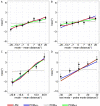
Results of Experiments 1–4. The plots show the adjustment bias as a function of mode–mean distance in (A) Experiment 1, (B) Experiment 2, (C) Experiment 3, or as a function of distance between the modes of a test set and a sample set in (D) Experiment 4. Data points depict average observed biases. Error bars show standard error of the mean with between-subject variance removed following the Cousineau (2005) method. The lines show the model predictions averaged across participants. Note that in (D), the biases in conditions with the right- (squares) and left-skewed (triangles) test distributions are shown with different data point shapes. As some models predict the same biases, blue and red lines on (A) and red and green lines on (D) substantially overlap.

Figure 5.

Results of Experiments 1–4. The plots show change in the Akaike information criterion (ΔAIC) summed across participants for four models in (A) Experiment 1, (B) Experiment 2, (C) Experiment 3, and (D) Experiment 4. The smaller the ΔAIC, the more likely the model was.

Figure 6.

Two feature distributions (histograms) with similar mode–mean distance (≈20°) but different shapes and corresponding model population responses (blue curves) normalized by peak activation. The population responses are modeled for the σ_tuning = 40°. In (A), a distribution from Experiments 1 and 2 is shown; in (B) a distribution from Experiment 3 is shown. As can be seen, even though the mean–mode distance is the same, the peak population response (blue vertical line) is shifted away from the mean (dashed vertical line) much stronger in (B) than in (A).

Figure 7.

Orientation distributions used in Experiment 3. Only left-skewed distributions are shown in this example, whereas the whole design included the right-skewed distributions as well.

References

1. Allik, J., Toom, M., Raidvee, A., Averin, K., & Kreegipuu, K. (2013). An almost general theory of mean size perception. Vision Research, 83, 25–39, 10.1016/j.visres.2013.02.018. - DOI - PubMed
1. Ariely, D. (2001). Seeing sets: Representation by statistical Properties. Psychological Science, 12(2), 157–162. JSTOR. - PubMed
1. Ariely, D. (2008). Better than average? When can we say that subsampling of items is better than statistical summary representations? Perception & Psychophysics, 70(7), 1325–1326, 10.3758/PP.70.7.1325. - DOI - PubMed
1. Baek, J., & Chong, S. C. (2020a). Ensemble perception and focused attention: Two different modes of visual processing to cope with limited capacity. Psychonomic Bulletin & Review, 27, 1–5, 10.3758/s13423-020-01718-7. - DOI - PubMed
1. Baek, J., & Chong, S. C. (2020b). Distributed attention model of perceptual averaging. Attention, Perception, & Psychophysics, 82(1), 63–79, 10.3758/s13414-019-01827-z. - DOI - PubMed
Publication types