Bridging physiological and perceptual views of autism by means of sampling-based Bayesian inference

Abstract

Theories for autism spectrum disorder (ASD) have been formulated at different levels, ranging from physiological observations to perceptual and behavioral descriptions. Understanding the physiological underpinnings of perceptual traits in ASD remains a significant challenge in the field. Here we show how a recurrent neural circuit model that was optimized to perform sampling-based inference and displays characteristic features of cortical dynamics can help bridge this gap. The model was able to establish a mechanistic link between two descriptive levels for ASD: a physiological level, in terms of inhibitory dysfunction, neural variability, and oscillations, and a perceptual level, in terms of hypopriors in Bayesian computations. We took two parallel paths-inducing hypopriors in the probabilistic model, and an inhibitory dysfunction in the network model-which lead to consistent results in terms of the represented posteriors, providing support for the view that both descriptions might constitute two sides of the same coin.

Keywords: Autism; Hypopriors; Inhibitory dysfunction; Neural circuits; Sampling-based inference.

Figure 1.

Sketches of the generative model, and a neural circuit implementing sampling-based probabilistic inference under that model. (A) The Gaussian scale mixture (GSM) generative model. Under this model, each image patch is built as a linear combination of local features (projective fields), whose intensities are drawn from a multivariate Gaussian distribution. This linear combination is then further scaled by a global contrast level and subject to noise. The features were in this case a set of localized oriented Gabor filters that differed only in their orientations and were uniformly spread between −90° and 90°. The image serving as stimulus in the figure is for illustration only. Photo credit: Santa Fe Bridge by Enzo Ferrante (https://eferrante.github.io/). (B) A 2D projection of the posterior distribution for a given a visual stimulus as computed by the Bayesian ideal observer under the GSM. (C) The recurrent E–I neural network receives an image patch as an input, which is filtered by feedforward receptive fields matching the projective fields of GSM in panel A. Each latent variable in the GSM is represented by the activity of one E cell in the network. (D) A 2D projection of the neural responses of E cells corresponding the same 2 latent variables shown in panel B. Over time, the network samples from the posterior distribution corresponding to the stimulus it receives.

Figure 2.

Inference under the GSM and responses in the original network, here representing healthy neurotypical subjects. Replotted from Echeveste et al. (2020). In all panels, shades of green correspond to the ideal observer, while red corresponds to network responses, as in Figure 1. Line colors in panel B indicate different contrast levels, which are the same as stimulus frames in panel A, indicating to which stimulus responses correspond. (A) Stimuli (shade of frame color indicates contrast level, split green, blue, and red indicate that the same stimuli were used as input to the ideal observer and to both neural networks). (B) Covariance ellipses (2 standard deviations) of the ideal observer's posterior distributions (green) and of the networks' corresponding response distributions (red). Red trajectories show sample 500-ms sequences of activities in the networks. As in the sketch of Figure 1, 2D projections corresponding to two representative latent variables / excitatory cells are shown. These two correspond to projective fields / receptive fields at preferred orientations 42° and 16°. (C) Mean (top) and standard deviation (bottom) of latent variable intensities ordered by each latent's orientation, for each stimulus in the training set. Left: from the ideal observer's posterior distribution (green). Right: E cell membrane potentials u_E from the networks' stationary distributions (red). Response moments in panel C were estimated from n = 20,000 independent samples (taken 200 ms apart).

Figure 3.

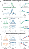
Hypopriors and impaired inhibition. (A, B) Effect of hypopriors on posterior predictions for a 1D toy example. Priors, likelihoods, and posteriors are all Gaussian. A contrast variable regulating the likelihood precision plays the role of the perceptual reliability of stimuli. Two example inference cases are presented: under the true (well-calibrated) prior (dashed, green) and under a wider hypoprior (dashed, blue). (A) The prior (dashed, color) and likelihood (dashed, black) are multiplicatively combined according to Bayes’ rule to form the posterior (continuous, color). (B) Posterior mean (top plot) and standard deviation (bottom plot) under the true prior (green) and the hypoprior (blue), as a function of contrast (likelihood precision). (C, D) Effect of hypopriors on posterior predictions for the full multivariate GSM model. (C) Mean (top plots) and standard deviation (bottom plots) of latent variable intensities ordered by each latent’s orientation, for each stimulus in Figure 2. Left: for the well-calibrated ideal observer’s posterior distribution (green). Right: under a hypoprior (blue). (D) Posterior mean (top) and standard deviation (bottom), averaged across all latent variables, under the true prior (green) and the hypoprior (blue), as a function of contrast. (E, F) Effect of impaired inhibition on network responses. (E) Mean (top) and standard deviation (bottom) of latent variable intensities ordered by each latent’s orientation, for each stimulus in the training set. E cell membrane potentials u_E from the stationary response distributions for the NT-network (left, red), and for the ASD-network (right, blue). (F) Mean (top) and standard deviation (bottom) of neural responses, averaged across all cells, for the NT-network (red) and the ASD-network (blue), as a function of contrast. Circles, and gray dots on x-axis of panels D and F indicate training contrast levels.

Figure 4.

Transient responses and oscillations. (A) LFP power as a function of frequency for stimuli of different contrast levels (same stimuli and colors as in Figure 3) in the NT-network (left), and in the ASD-network (right). Both networks present strong gamma oscillations (see peaks in the gamma band, indicated by empty circles). (B) Comparison of oscillatory behavior in both networks. On the left, the peak gamma frequency is presented as a function of stimulus contrast for both networks. Very minimal differences are observed. On the right, the total power within the gamma band is presented as a function of contrast for both networks. A higher gamma power is observed for the ASD-network at all contrasts, with strong differences at low contrasts. (C) Across-trial average transient responses for stimuli of different contrast levels in the neurotypical network (left) and in the ASD-network (right). Both networks present strong stimulus-dependent transient overshoots. (D) Comparison of overshoot sizes. The maximal firing rate is presented as a function of stimulus contrast for both networks. We observe that the ASD-network presents stronger peak responses at higher contrasts, overreacting to intense stimuli. NT-network results reproduced from Echeveste et al. (2020).

References

1. Ahmadian, Y., Rubin, D., & Miller, K. (2013). Analysis of the stabilized supralinear network. Neural Computation, 25(8), 1994–2037. 10.1162/NECO_a_00472, - DOI - PMC - PubMed
1. Aitchison, L., & Lengyel, M. (2016). The Hamiltonian brain: Efficient probabilistic inference with excitatory-inhibitory neural circuit dynamics. PLoS Computational Biology, 12(12), e1005186. 10.1371/journal.pcbi.1005186, - DOI - PMC - PubMed
1. Aitchison, L., & Lengyel, M. (2017). With or without you: Predictive coding and Bayesian inference in the brain. Current Opinion in Neurobiology, 46, 219–227. 10.1016/j.conb.2017.08.010, - DOI - PMC - PubMed
1. American Psychiatric Association. (2013). Diagnostic and statistical manual of mental disorders (DSM-5). American Psychiatric Association Publishing. 10.1176/appi.books.9780890425596 - DOI
1. Aronov, D., Nevers, R., & Tank, D. W. (2017). Mapping of a non-spatial dimension by the hippocampal-entorhinal circuit. Nature, 543(7647), 719–722. 10.1038/nature21692, - DOI - PMC - PubMed
LinkOut - more resources