One dimensional approximations of neuronal dynamics reveal computational strategy

Abstract

The relationship between neuronal activity and computations embodied by it remains an open question. We develop a novel methodology that condenses observed neuronal activity into a quantitatively accurate, simple, and interpretable model and validate it on diverse systems and scales from single neurons in C. elegans to fMRI in humans. The model treats neuronal activity as collections of interlocking 1-dimensional trajectories. Despite their simplicity, these models accurately predict future neuronal activity and future decisions made by human participants. Moreover, the structure formed by interconnected trajectories-a scaffold-is closely related to the computational strategy of the system. We use these scaffolds to compare the computational strategy of primates and artificial systems trained on the same task to identify specific conditions under which the artificial agent learns the same strategy as the primate. The computational strategy extracted using our methodology predicts specific errors on novel stimuli. These results show that our methodology is a powerful tool for studying the relationship between computation and neuronal activity across diverse systems.

Fig 1. Schematic of LOOPER—A method for constructing simple models of nonlinear dynamical systems based on experimental observations.

Overview: A) Activity of a hypothetical system given by three neurons. The state of this system is characterized by the neuronal population activity vector, which records the instantaneous firing of all neurons (Neurons 1, 2 and 3). Note that the activity is confined to a helical manifold. Time is implicit and flows in the direction indicated by arrows in A through F. In this example, neuronal activity is recorded under three different task conditions shown by color in A-F. B) Diffusion mapping is used to unwrap the helical structure in A to reveal a simpler (2D) projection that contains all of the neuronal activity. While the unwrapped space is 2-dimensional, the actual dynamics of the system are largely confined to a set of three one dimensional trajectories each starting from a unique set of initial conditions (red, green and blue circles). So long as trajectories stay separate, the information stored in the state of the system is preserved. At the moment when red and blue trajectories merge, the system is no longer able to distinguish them (blue arrow). The merging of the trajectories can be quantified by the overlap in the distributions of neuronal activity (marginal histograms). On the contrary, the green trajectory is separated from the rest at the end of the trial. Thus, the distribution of the green points is distinct from the other two. C) Shows a diffusion map, normalized as a transition probability matrix, constructed from the observations in A. The three task conditions (three trials of each) are shown by three colored squares. The most likely transitions in each case are along the one off diagonal of the matrix. This corresponds to the actual observations. High transition probabilities away from this main diagonal correspond to similar dynamics observed on different trials. Note that the off diagonal bands appear late in the trials for blue and red conditions. In contrast, the green and red conditions are initially similar but diverge towards the end of the trial. D) Observations in C naturally inform a way to coarse grain the diffusion map. States characterized by similar transition probabilities (rows of the matrix in C) can be readily aggregated. This results in a course grained transition probability matrix where each entry is a cluster of experimental observations aggregated on the basis of similarity of rows in the diffusion map in C. This coarse grained transition probability matrix is shown as a graph. The position of each state (S1, S2, S2…) in the latent space is given by the mean of all experimental observations that comprise the state. Note that in this example transitions from each state (arrows) are predominantly to a single other state. This expresses the assumption that the most salient information can be represented by one dimensional trajectories. This assumption allows further simplification of the system by clustering states (S1, S2, …) into trajectories (ordered sequences of states). E) Finally, states within each trajectory are interpolated to reveal a model that consists entirely of one dimensional trajectoriess (each colored surface is a distinct trajectory). The width of each trajectory shows the variance of the experimental observations projected onto the latent space F) A useful way to describe the data is the “computational scaffold” which is the trajectory ID assigned to the observed data at each time point. Note that the data tends to separate out the initial conditions (red, green and blue) during the middle of the trial based on trajectory ID. Further, the way that the trajectories merge and split can give valuable insight into the types of information used by the system.

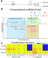
Fig 2. LOOPER model makes specific predictions about behaviour on novel stimuli combinations.

A) Schematic of the working memory task. We model our task on the Romo task [35]. In their task the monkey receives a sequence of two vibrational stimuli applied to the fingertip (F1 and F2), with an interstimulus delay of 3s. The monkey must push one of the two buttons depending on whether the frequency of F1 is greater than F2, or not. We trained an RNN consisting of 100 LSTM units to solve this task using the same statistics of stimuli as found in the original paper. For the RNN, stimuli are presented for 10 frames. Gaussian noise was added to both the input values, and the hidden states of the RNN. In order to compare to monkey data we include only the three F1 values that had more than 10 recordings for each neuron. B) The computational scaffold of the RNN solution has 3 parts. The system encodes and stores the values of F1 in the blue region. Note, however, that the trajectories representing F1 = 20 and F1 = 40 fuse before the onset of F2. The network is still able to complete the task because all F2s that follow F1 = 20 and F1 = 40 are distinct. This means that the network uses only the information about F2 (orange region) to solve the task. For the case of F2 = 15, however, the response of the system must vary depending on whether F1 = 10 or F1 = 20. Thus, the system must differentiate F1 = 10, and use that information to compare to F2 in the green region. C) Table of classification accuracies for both training and novel stimuli pairs. The computational scaffold in B predicts that the network will give erroneous results on the novel stimuli marked in red. The observed pattern of errors matches those predicted by LOOPER (top row), and confirms the assertion that the RNN fails to distinguish between F1 = 20 and F1 = 40 (as in B). A simulation of the LOOPER model fit to this network yields the same errors as the network (middle row). These error do not occur in an RNN trained on a modified dataset (Fig 3) in which the exploit cannot occur (bottom row).

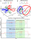
Fig 3. Computational scaffold is conserved between monkey and RNN despite disparate neuronal activity patterns.

Mean subtracted activity in prefrontal cortex (A) and RNN (B) projected onto the first three principal components (56% variance explained in monkey, 83% explained in RNN). Thin lines show observed neuronal activity on a single trial (colored by task condition). Stable trajectories extracted by LOOPER are also projected onto these PCs(thick lines). Dashed lines indicate F1 < F2 and solid lines indicate F1 > F2. Shaded area reflects the variance of the data assigned to each model bin. The F1 and F2 stimulus timings are shown as white markers. Black arrows show phase velocity. Computational scaffolds constructed using LOOPER on monkey (C) and RNN (D) data. Both the RNN and monkey share the same number of trajectories and branching patterns, implying that they have the same computational scaffold. F1 causes the system to diverge into 3 distinct trajectories (Encode and store F1). F2 causes each of those trajectories to bifurcate (Compare stored F1 to F2). Note that the same F2 maps onto different trajectories depending on the value of F1. Thus, unlike F1 which is stored in the system dynamics, F2 information does not map onto a unique trajectory.

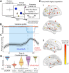
Fig 4. Computational scaffold of neuronal dynamics extracted using LOOPER predicts choices on the theory of mind task.

A) Schematic of the “human theory of mind” task. Subjects are shown videos of shapes moving on the screen and are asked whether the shapes are having a mental interaction or not. We build the LOOPER model on only those trials in which the subjects answered either “Yes” or “No”. B) Validation trials excluded from model construction are projected onto their closest model bin at each time step. A stereotypical example of the computational scaffold. Each trial in the validation set is colored by whether the subject responded that “Yes, they do think there was an interaction” (orange traces), or “No, they don’t think there was an interaction” (blue traces). Notice that the two conditions diverge near the end of the movie and during the response window. This is consistent with accumulation of information throughout the movie that eventually culminates in a binary decision (validation accuracy 98.8%, n = 1000). C) Due to the high amount of noise in the fMRI signal the exact timings of divergence of trajectories is parameter dependent. To ensure that our result is robust with respect to parameter choices, we explore the effect of parameter values on the computational scaffold. The average number of trajectories and the 95% confidence interval is plotted at each time point. D) Accuracy of decoding the response using LOOPER and standard supervised techniques used in fMRI literature (SVM). All reported accuracies are on the validation dataset. The baseline SVM classifier used the same training data as LOOPER (10 trials of each condition bootstrapped over 60 subjects). For LOOPER, the raw parcel time series were used. For SVM, the data were subjected to PCA (top 20 PCs, 98% variance explained) and averaged over time. The baseline model (orange) averages over the full trial time. Classification accuracy is vastly improved by using the top 20 PCs calculated on the basis of both the training and validation datasets (yellow). Accuracy is further improved by taking the average over the period of separation found by LOOPER (B and C) instead of over the full trial (purple). However, none of these models perform at the same level as the LOOPER model (p < 0.001). We can recover LOOPER-level accuracies by dramatically increasing the number of trials fed into the SVM (green). E) Visualization of the most sensitive parcels during the time of divergence of the two conditions (responded “Yes” or “No”). We generate 100 random sets of trials using the same bootstrapping paradigm as used to build the LOOPER model. For each set of trials we find the maximum sensitivity index, d’, for each parcel during the time of interest and take the median of these maximum d’ values over the 100 iterations of trials. The top 20 brain regions are plotted.

Fig 5. LOOPER model explains majority of variance and predicts future neuronal activity.

Simple models obtained using LOOPER are remarkably good at reconstructing the dynamics observed in diverse systems such as artificial recurrent neural networks (A), whole brain calcium imaging in C. elegans during spontaneous locomotion (B), visually evoked local field potentials in the mouse (C), firing of neurons in prefrontal cortex of a primate during working memory task (D), and BOLD signals in humans performing a “theory of mind task” (E). Top panels in (A-E) are experimental observations (red vertical lines show different trials or stimuli timings). Bottom panels are LOOPER reconstruction of the observed activity. R² values are calculated between each observed trial (i.e. #channels x time matrix) and the corresponding reconstructed trial. We also include the number of PC components required to achieve an equivalent R² in the parentheses. LOOPER models preserve the majority of variance in the data across a vast variety of systems and signal types. LOOPER is also able to predict future neuronal activity of the systems (F-I). Black lines are either a single trial (RNN) or a bootstrapped sample of several trials (mouse → 5 trials; monkey → 10 pseudo trials (see main text); BOLD signals → 60 trials). Top four panels show examples of four recording channels (total of 100 LSTM units, 49 electrodes in mouse, 179 neurons in monkey and 264 parcels in human). Red lines show an average of 100 simulations of the LOOPER model (shaded area shows standard deviation). The bottom panels show the distribution of correlation coefficients computed across multiple bootstrap subsets (or individual trials) and recording channels. For each experimental system, the LOOPER model is constructed on a subset of trials. Validation trials (or bootstrapped averages) are constructed from a non-overlapping subset of trials. Each simulation begins at the same timepoint in the trial (beginning of solid black line). The initial conditions for the LOOPER simulation are given by the closest model bin to the observed neuronal activity at this time. The dynamics starting from these initial conditions given by the LOOPER model are simulated and projected back into observation space for comparison to experimental observations. Note that the simulation periods are chosen such that no task-relevant stimuli are present, and so no input is required for the simulations. Correlation is computed over the period of the simulation starting from t₀ and continuing for several time steps (RNN → 40 time steps, mouse → 50 time steps, monkey → 19 time steps, human → 20 time steps). Median correlation values are RNN → 0.98, mouse → 0.79, monkey → 0.95, human → 0.62, (J-M, blue box, left). We also compared LOOPER’s simulations to simulations using conventional HMMs using the same methodolgy as above (J-M, orange box, left). Finally, we used both the LOOPER and HMM models to attempt to decode the state of the system at each point in time and task condition. The task decoding rate is the average difference between the model’s decoding rate and the expected decoding rate given the task (Romo task: 50% during the interstimulus period and 100% after the presentation of F2, Theory of Mind task: 100% during the period of separation in Fig 4B). Average decoding rates are shown in Fig 5J–5M (blue and orange boxes, right). Chance level decoding rate given a uniform distribution null model of the Romo task is 25%, and for the Theory of Mind task it is 50%. Note that the mouse data has no associated task and so is left blank.

References

1. Hubel DH, Wiesel TN. Receptive fields and functional architecture of monkey striate cortex. The Journal of Physiology. 1968;195(1):215–243. doi: 10.1113/jphysiol.1968.sp008455 - DOI - PMC - PubMed
1. Moser EI, Kropff E, Moser MB. Place Cells, Grid Cells, and the Brain’s Spatial Representation System. Annual Review of Neuroscience. 2008;31(1):69–89. doi: 10.1146/annurev.neuro.31.061307.090723 - DOI - PubMed
1. Nieh EH, Schottdorf M, Freeman NW, Low RJ, Lewallen S, Koay SA, et al.. Geometry of abstract learned knowledge in the hippocampus. Nature. 2021;595(7865):80–84. doi: 10.1038/s41586-021-03652-7 - DOI - PMC - PubMed
1. Michaels JA, Dann B, Scherberger H. Neural population dynamics during reaching are better explained by a dynamical system than representational tuning. PLoS computational biology. 2016;12(11):e1005175. doi: 10.1371/journal.pcbi.1005175 - DOI - PMC - PubMed
1. Mante V, Sussillo D, Shenoy KV, Newsome WT. Context-dependent computation by recurrent dynamics in prefrontal cortex. nature. 2013;503(7474):78–84. doi: 10.1038/nature12742 - DOI - PMC - PubMed
Publication types