Behavioral origin of sound-evoked activity in mouse visual cortex

Abstract

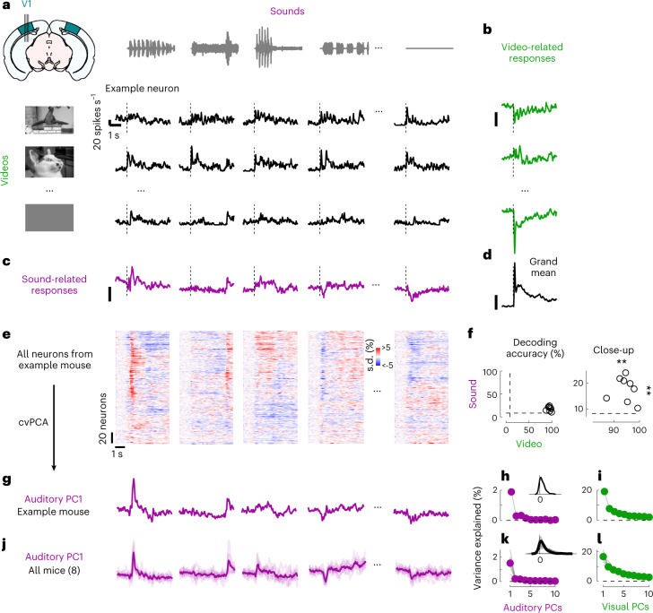
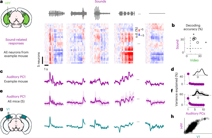
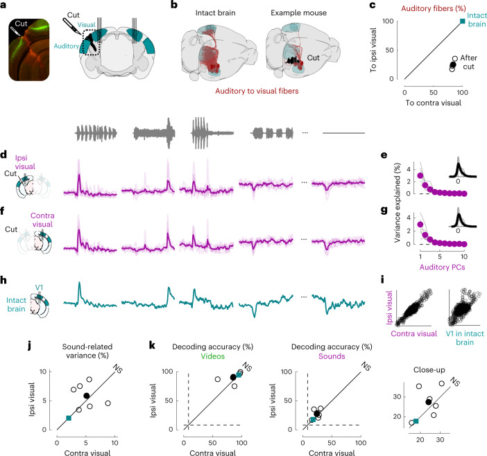
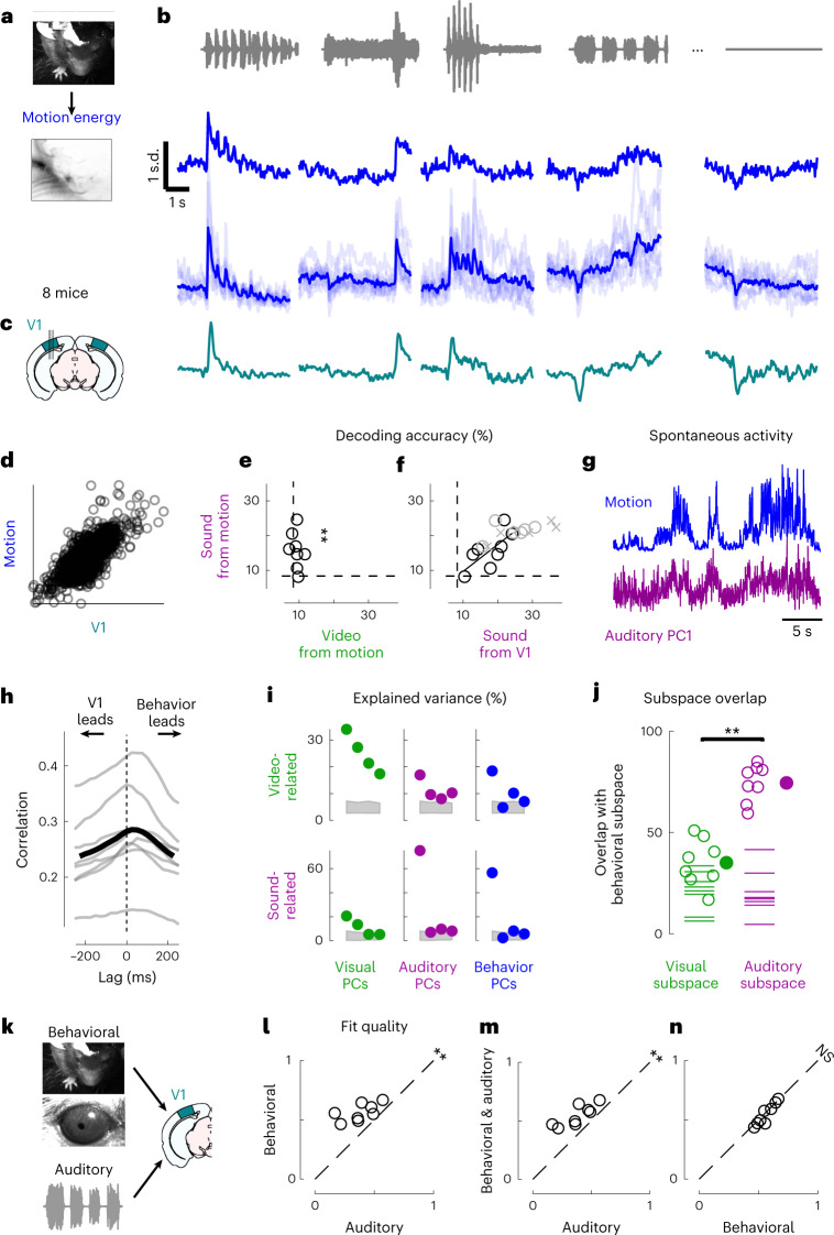
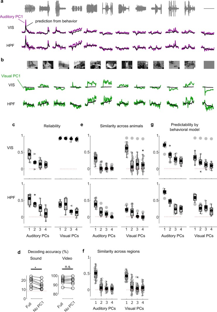
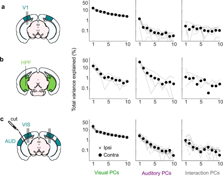
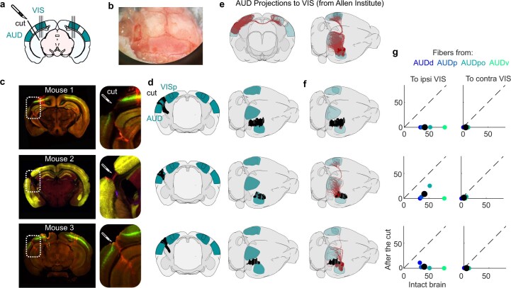
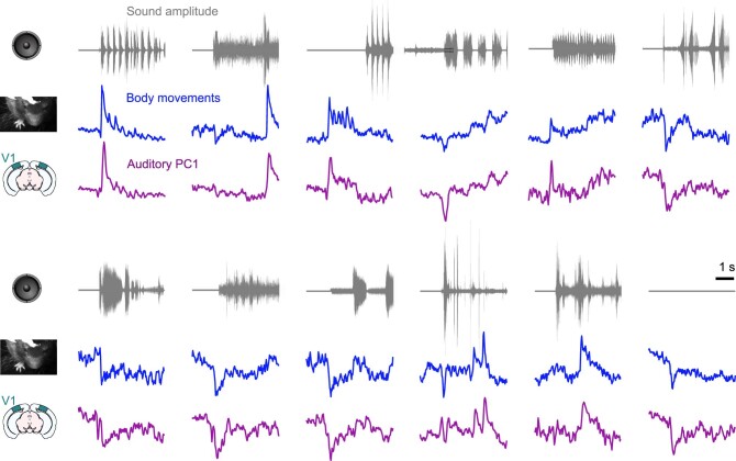
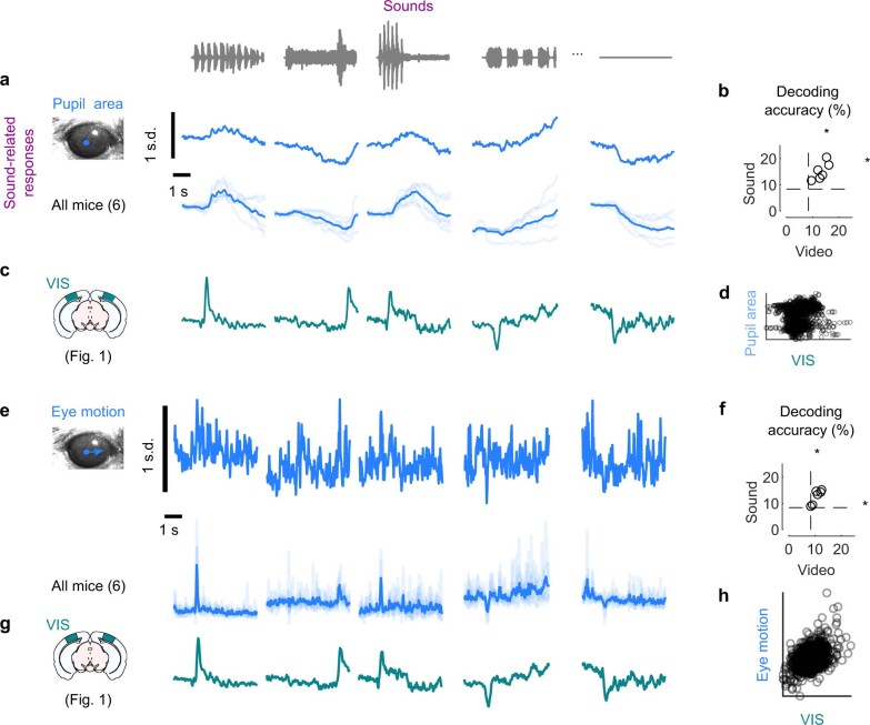
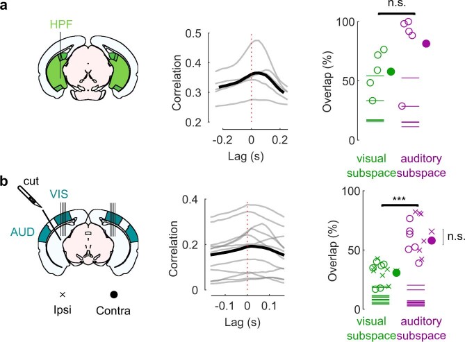
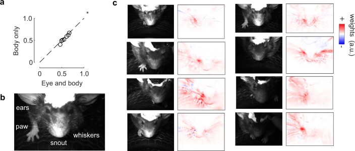
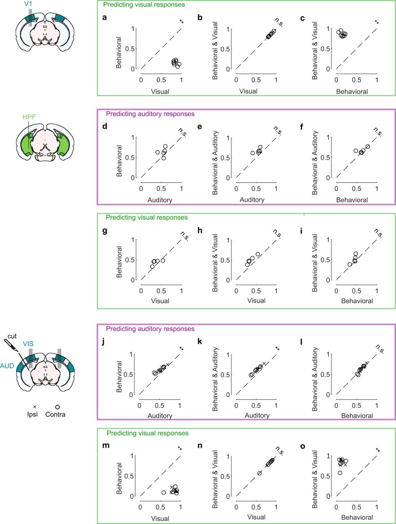
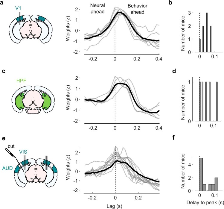
Sensory cortices can be affected by stimuli of multiple modalities and are thus increasingly thought to be multisensory. For instance, primary visual cortex (V1) is influenced not only by images but also by sounds. Here we show that the activity evoked by sounds in V1, measured with Neuropixels probes, is stereotyped across neurons and even across mice. It is independent of projections from auditory cortex and resembles activity evoked in the hippocampal formation, which receives little direct auditory input. Its low-dimensional nature starkly contrasts the high-dimensional code that V1 uses to represent images. Furthermore, this sound-evoked activity can be precisely predicted by small body movements that are elicited by each sound and are stereotyped across trials and mice. Thus, neural activity that is apparently multisensory may simply arise from low-dimensional signals associated with internal state and behavior.

Fig. 1. Sounds evoke stereotyped responses in visual cortex.

a, Responses of an example neuron to combinations of sounds (columns) and videos (rows). Responses were averaged over four repeats. b, Video-related time courses (averaged over all sound conditions, minus the grand average) for the example neuron in a. c, Same, for the sound-related time courses. d, Grand average over all conditions for the neuron. Scale bars in b–d: 20 spikes per second. e, Sound-related time courses for all 212 neurons in one experiment, sorted using rastermap. f, Decoding accuracy for video versus sound (double asterisks indicate P = 0.0039, Wilcoxon right-tailed signed rank test, n = 8 mice). Dashed lines show chance level (1/12). g, Time courses of the first principal component of the sound-related responses in e (‘auditory PC1’, arbitrary units). h, Fraction of total variance explained by auditory PCs, for this example mouse; inset: distribution of the weights of auditory PC1 (arbitrary units), showing that weights were typically positive. i, Same, for visual PCs. j–l, Same as g–i, for individual mice (thin curves) and averaged across mice (thick curves).

Fig. 2. Sounds evoke stereotyped responses in hippocampal formation.

a, Sound-related time courses for all 28 neurons in HPF in one experiment, sorted using rastermap. b, Decoding accuracy for video versus sound (asterisk indicates P = 0.031, Wilcoxon right-tailed signed rank test, n = 5 mice). Dashed lines show chance level (1/12). c, Time courses of the first principal component of the sound-related responses in a (‘auditory PC1’, arbitrary units). d, Fraction of total variance explained by auditory PCs, for this example mouse; inset: distribution of the weights of auditory PC1 (arbitrary units). e,f, Same as c and d for individual mice (thin curves) and average of all mice (thick curves). g, Time courses of the auditory PC1 in visual cortex (from Fig. 1), for comparison. h, Comparison of the auditory PC1 from HPF (from e) and from V1 (from Fig. 1); arbitrary units.

Fig. 3. Sound responses in visual cortex are not due to inputs from auditory cortex.

a, Coronal views of a transectomy cutting the connections between auditory and visual cortex in one hemisphere, showing histology (left) and reconstruction of the cut (right). After the cut, bilateral recordings are performed in visual cortex. b, Three-dimensional visualizations showing auditory to visual fibers (red) in an intact brain (top) versus after the cut (bottom) in an example mouse. c, Auditory input to the sides contralateral versus ipsilateral to the cut for all three mice (open dots) and their average (filled dot), normalized by the input expected in intact brains (turquoise dot). d, Time courses of the first principal component of the sound-related responses (‘auditory PC1’) on the side ipsilateral to the cut (average over all mice). Thin curved lines show individual mice. e, Fraction of total variance explained by auditory PCs on the side ipsilateral to the cut; inset: distribution of the weights of auditory PC1 for all mice. f,g, Same as d and e for the side contralateral to the cut. h, Time courses of the auditory PC1 in visual cortex of intact, control mice (from Fig. 1) for comparison. i, Comparison of the auditory PC1 from the sides contralateral and ipsilateral to the cut (left, from d versus f) and from V1 (right, taken from b versus Fig. 1); all arbitrary units. j, Sound-related variance explained by the first four auditory PCs on the ipsi- versus contralateral side, showing individual sessions (open dots), their average (black dot) and the average across control mice (turquoise dot) (Wilcoxon two-sided paired signed rank test, n = 6 sessions across three mice). k, Decoding accuracy for videos (left) and sounds (middle and right, showing close-up) (Wilcoxon two-sided paired signed rank test, n = 6 sessions across three mice). Symbols are as in j.

Fig. 4. Sounds evoke stereotyped, uninstructed behaviors that predict sound responses in visual cortex.

a, Extraction of motion PCs from videos of the mouse face. b, Sounds evoked changes in the first motion PC, both in an example mouse (top) and all mice (bottom). Scale bar: 1 s.d. c, Time courses of the auditory PC1 in visual cortex (from Fig. 1). d, Comparison of the time courses of motion (taken from b) and of the auditory PC1 from V1 (taken from Fig. 1); all arbitrary units. e, Decoding of sound identity from the first 128 motion PCs was significantly above chance level (dashed lines) (double asterisks indicate P = 0.0078, Wilcoxon right-tailed signed rank test, n = 8 mice). f, Across mice, there was a strong correlation between the accuracy of sound decoding from facial motion and from V1 activity. The linear regression is performed on the control mice from Fig. 1 (black dots). Data from transectomy mice (gray markers) confirm the trend, both on the cut side (crosses) and on the uncut side (circles). g, Time course of facial motion (top) and of V1 activity along auditory PC1 (bottom) in the absence of any stimulus, for an example mouse. h, Cross-correlogram of these time courses, for individual mice (gray) and their average (black). The positive lag indicates that movement precedes neural activity. i, Video- and sound-related variance explained by neural activity along the visual (left), auditory (middle) or behavioral (right) subspaces (first four PCs of each subspace), for one example mouse. The gray regions show 90% confidence intervals expected by chance (random components). j, Overlap between the auditory or the visual subspace and the behavioral subspace for each mouse (open dots) and all mice (filled dot) (double asterisks indicate P = 0.0078, Wilcoxon two-sided paired signed rank test, n = 8 mice). Dashed lines show the significance threshold (95th percentile of the overlap with random dimensions) for each mouse. k, Schematics of the three encoding models trained to predict the average sound-related activity in the auditory subspace. l–n, Cross-validated correlation of the actual sound responses and their predictions for all mice, comparing different models (auditory, behavioral and full; double asterisks indicate P = 0.0078, Wilcoxon two-sided paired signed rank test, n = 8 mice).

Extended Data Fig. 1. Coding of visual vs. auditory stimuli in visual cortex and hippocampal formation.

a. Time courses of the auditory PC1 averaged across mice (z-scored), measured in visual cortex (VIS, top) and hippocampal formation (HPF, bottom). Traces show the actual data (purple) and the cross-validated prediction from the behavioral model (black). b. Same as a, but for visual PC1 (green). c. Reliability of each auditory (left) or visual (right) PC, in VIS (top, n = 8 mice) or HPF (bottom, n = 5 mice). The large dot shows the z-transformed mean; the bounds of each box show the 25^th and 75^th percentiles; the whiskers show the minimum and maximum values that are not outliers; small dots show outliers (computed using the interquartile range); individual dots are also shown. d. Decoding accuracy of sound identity from auditory PCs (left) or video identity from visual PCs (right) measured in VIS, taking the full subspace or the full subspace except PC1. Sound decoding was significantly worse without auditory PC1 (*: p = 0.0156, two-sided paired Wilcoxon sign rank, n = 8 mice). e. Same as c but showing the similarity across animals. Reliability of each PC is shown for reference (gray, replotted from c). f. Similarity of visual and auditory PCs between VIS and HPF. g. Same as e, for the predictability of each PC by the behavioral model, measured by the cross-validated correlation between data and model prediction. The model can sometimes predict the test set better than the train set because it can predict fluctuations specific to the test set.

Extended Data Fig. 2. Dimensionality of auditory and visual responses in visual cortex and hippocampal formation.

a. Top: Total variance explained (normalized test-retest covariance) for visual PCs (left), auditory PCs (middle) and interactions PCs (right), for all 8 recordings in V1 (thin lines) and their average (filled dots). The total variance is measured from the normalized test-retest covariance, which can occasionally be negative (not visible in logarithmic scale). b. Same as a but with the 5 recordings from the HPF. c. Same as a but with the 12 recordings from the visual cortices ipsilateral (6, crosses) and contralateral (6, filled dots) to the cut (6 sessions across 3 mice).

Extended Data Fig. 3. Transectomy cut most of the fibers from auditory to visual cortex.

a. Schematic of the transectomy experiments: the connections between auditory (AUD) and visual (VIS) cortex are cut on one side. Subsequently, recordings are performed in visual cortex, in both hemispheres. b. Picture from above of the mouse skull during surgery, with a craniotomy performed on the left side. c. Histology of the three mouse brains, showing the cut (inset), and the probe tracks (DiI and DiO staining, mainly visible in mice 1 and 3). d. 3D reconstructions of the cut, shown from a coronal view (left) or from above/sideways (right). e. Fiber tracks from the auditory cortex to the visual cortex in intact mice, from 53 experiments performed in the Allen Mouse Brain Connectivity atlas, see Methods). f. Estimated intact fibers after the cut, for the 3 mice. g. Estimate of the number of fibers before the cut (abscissa) and after the cut (ordinate) for each mouse, in ipsilateral (left) and contralateral visual cortex (right). The color of the dots indicates the auditory area from which the fibers originated (Allen Mouse Brain Connectivity Atlas). The black dot shows the average over all 53 experiments performed for the Atlas.

Extended Data Fig. 4. Neural and behavioral responses differ across sounds but resemble each other.

Responses along neural auditory PC1 from V1 (purple), and motion energy (blue) for all sounds. Responses are averaged over repeats, videos, and mice, and z-scored. The top trace (gray) shows the envelope of the corresponding sound. As in all main text figures, these responses are expressed relative to the grand average over sounds and videos; this explains the negative deflections seen in the responses to the blank stimulus.

Extended Data Fig. 5. Sounds trigger changes in arousal and eye movements.

a. Sound-related responses changes in arousal as measured by pupil diameter, for one example mice, and all mice (6 of 8 were monitored with an eye camera). b. Decoding of video and sound identity using pupil area. (*: p = 0.0156, right-tailed Wilcoxon sign rank test, n = 6 mice) c. Comparison with the time course of the neural auditory PC1 from Fig. 1. d. Scatter plot of auditory PC1 vs. pupil area. f-h. Same as a-d. but for eye movements (in f, *: p = 0.0312 for videos and 0.0156 for sounds).

Extended Data Fig. 6. Timing of movements and sound-related neural activity and overlap between neural subspaces related to behavior and sounds.

a. Left: Cross-correlogram of the motion energy and the neural activity on the auditory PC1 during the spontaneous period, for individual mice (gray) and averaged across mice (black). A positive lag means that movement preceded neural activity. Right: Overlap between the neural subspace related to behavior and the subspace related to video (left) or to sound (right), for each mouse (open dots) and averaged across mice (filled dot). Dashed lines show the significance threshold (95^th percentile of the overlap with random dimensions) for each mouse (two-sided paired Wilcoxon sign rank test, n = 5 mice). b. Same as a for the recordings in visual cortex after a transectomy (***: p = 0.00048, two-sided paired Wilcoxon sign rank test, n = 12 recordings across 3 mice; comparison cut vs. uncut side: two-sided paired Wilcoxon sign rank test, n = 6 sessions across 3 mice).

Extended Data Fig. 7. Sound-evoked V1 responses are mainly explained by whisker movements.

a. Correlation of the actual data and their predictions for all mice, comparing a model containing both eye and body movements predictors (‘Eye and body’) to a model containing only body movements predictors (‘Body only’). The eye predictors only marginally increase the fit prediction accuracy (*: p = 0.039, two-sided paired Wilcoxon sign rank test, n = 6 mice), suggesting that body movements are the best and main predictors. b. Example frame of the face, with the parts of the body that were visible. c. For each mouse, we analyzed the image of the mouse (left) and obtained the weights that best predicted the auditory PC1 (right). Most of the weights are related to the whiskers. The asymmetry of the weight distribution across the two sides of the face is likely due to differences in lighting.

Extended Data Fig. 8. Movements predict activity evoked by sounds in visual cortex and HPF, and by videos in HPF.

a-c. Cross-validated correlation of the visual responses and their predictions for all mice, comparing 3 different models: one with videos only (‘Visual’), one with eye and body movements only (‘Behavioral’), and one with all predictors (‘Full’) (**: p = 0.0078, n = 8 mice). d-f. Same as a-c but for auditory responses for the HPF recordings (albeit the low number of animals did not allow for conclusions on significance). (n = 5 mice) g-i. Same as a-c but for visual responses for the HPF recordings. j-l. Same as a-c but for auditory responses for the transectomy experiment recordings (**: p = 0.00049, n = 12 recordings across 3 mice). m-o. Same as a-c but for visual responses for the transectomy experiment recordings. All tests are two-sided paired Wilcoxon sign rank test.

Extended Data Fig. 9. Sound-evoked body movements and sound-evoked brain activity fluctuate together.

a. Single-trial, sound-related activity along auditory PC1 for one example mouse (purple). The prediction from the auditory model (gray) and the behavioral model (blue) are shown. b. Correlation between the single-trial noise in neural activity along auditory PC1 and the single-trial noise in the prediction for the same example mouse. c. Correlation values for all mice (open dots) and their average (filled dot).

Extended Data Fig. 10. Body movements precede brain activity.

a. Weights of the regression model to predict neural auditory PC1 from motion PCs (z-scored motion PC1 weights only are shown) for each individual mice (gray) and the average across mice (black). The model was computed on the spontaneous (no stimulus) period for the visual cortex experiments (Fig. 1). b. Distribution of the delay to the peak of the weights. A positive delay means that movement precedes and predicts neural activity by such a delay. c, d. Same as a, b, but for recordings in the HPF (Fig. 2). e,f. Same as a, b, but for recordings in visual cortex during the transectomy experiment (Fig. 3) (both sides).

References

1. Ghazanfar AA, Schroeder CE. Is neocortex essentially multisensory? Trends Cogn. Sci. 2006;10:278–285. doi: 10.1016/j.tics.2006.04.008. - DOI - PubMed
1. Iurilli G, et al. Sound-driven synaptic inhibition in primary visual cortex. Neuron. 2012;73:814–828. doi: 10.1016/j.neuron.2011.12.026. - DOI - PMC - PubMed
1. Ibrahim LA, et al. Cross-modality sharpening of visual cortical processing through layer-1-mediated inhibition and disinhibition. Neuron. 2016;89:1031–1045. doi: 10.1016/j.neuron.2016.01.027. - DOI - PMC - PubMed
1. Meijer GT, Montijn JS, Pennartz CMA, Lansink CS. Audiovisual modulation in mouse primary visual cortex depends on cross-modal stimulus configuration and congruency. J. Neurosci. 2017;37:8783–8796. doi: 10.1523/JNEUROSCI.0468-17.2017. - DOI - PMC - PubMed
1. Deneux T, et al. Context-dependent signaling of coincident auditory and visual events in primary visual cortex. eLife. 2019;8:e44006. doi: 10.7554/eLife.44006. - DOI - PMC - PubMed
Publication types