GliaMorph: a modular image analysis toolkit to quantify Müller glial cell morphology

Abstract

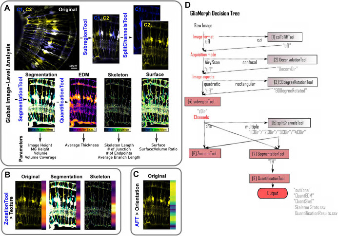
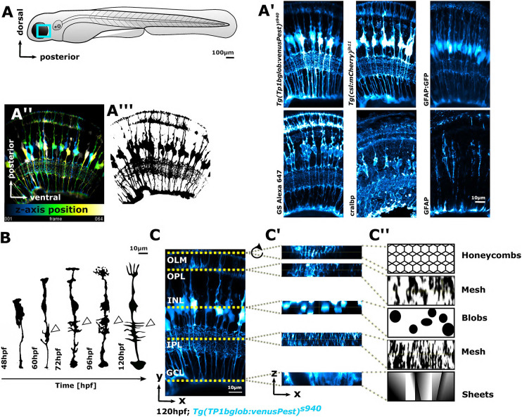
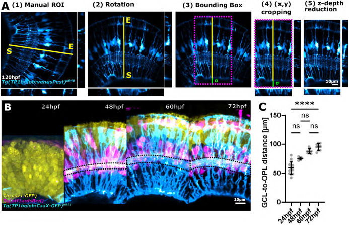
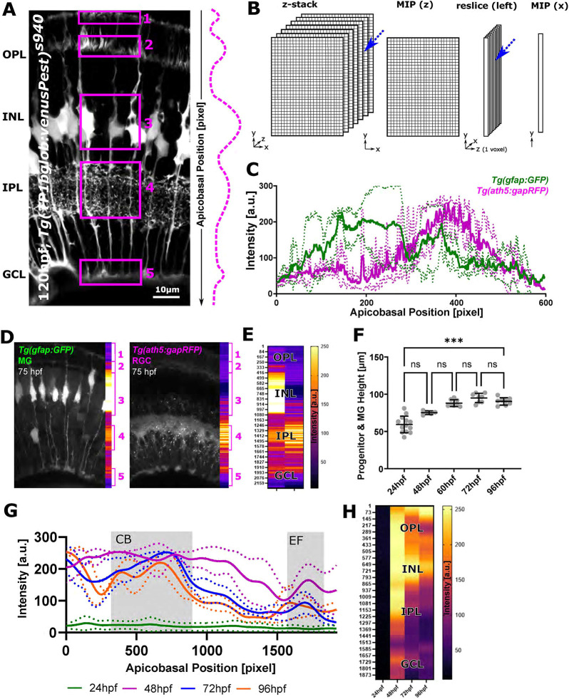
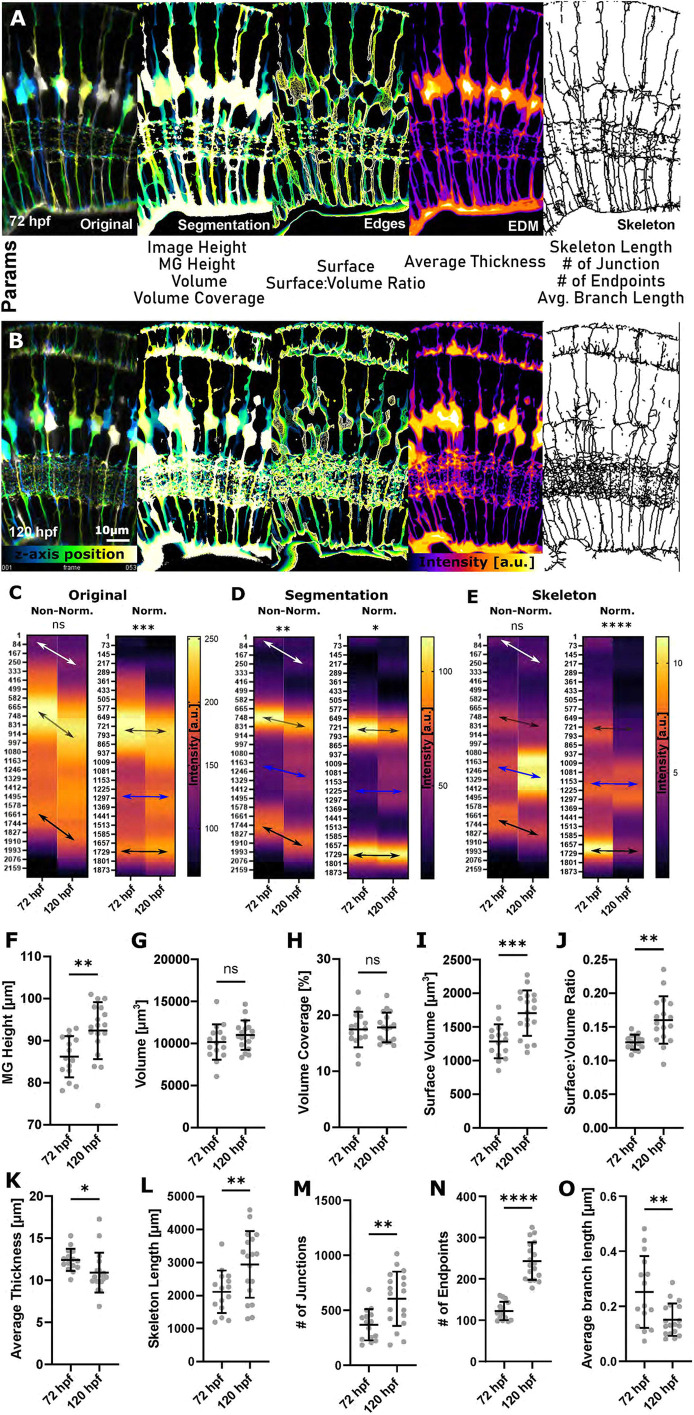
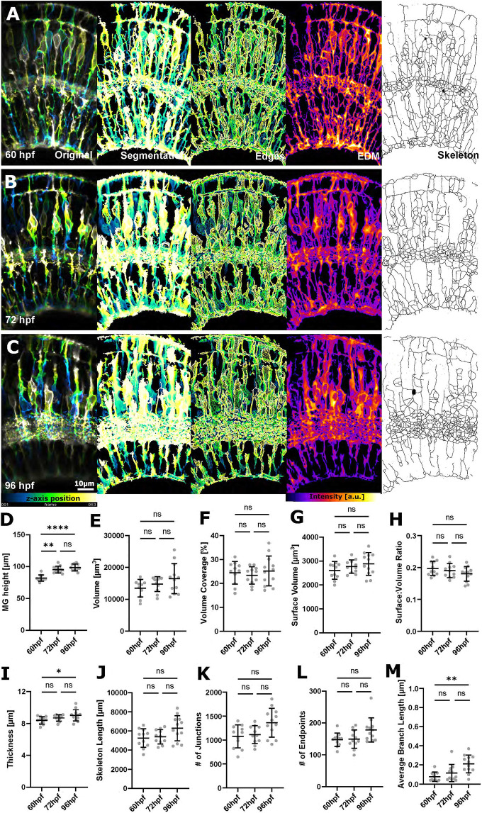
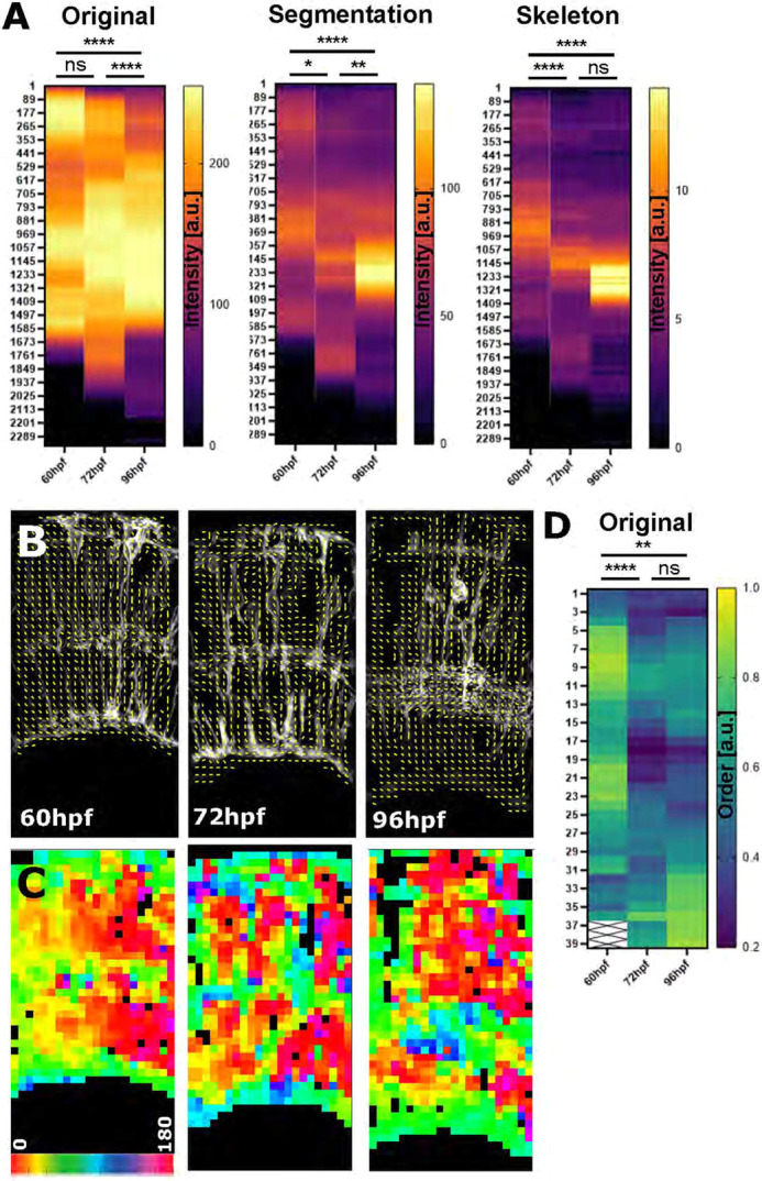
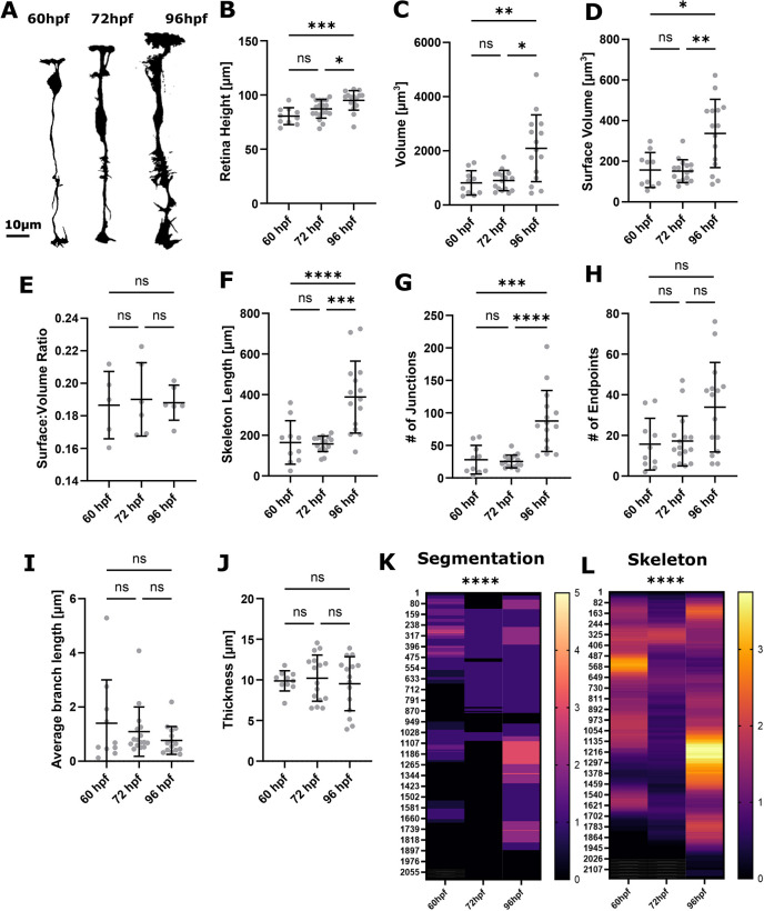
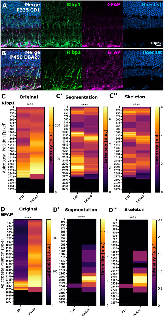
Cell morphology is crucial for all cell functions. This is particularly true for glial cells as they rely on complex shape to contact and support neurons. However, methods to quantify complex glial cell shape accurately and reproducibly are lacking. To address this, we developed the image analysis pipeline 'GliaMorph'. GliaMorph is a modular analysis toolkit developed to perform (1) image pre-processing, (2) semi-automatic region-of-interest selection, (3) apicobasal texture analysis, (4) glia segmentation, and (5) cell feature quantification. Müller glia (MG) have a stereotypic shape linked to their maturation and physiological status. Here, we characterized MG on three levels: (1) global image-level, (2) apicobasal texture, and (3) regional apicobasal vertical-to-horizontal alignment. Using GliaMorph, we quantified MG development on a global and single-cell level, showing increased feature elaboration and subcellular morphological rearrangement in the zebrafish retina. As proof of principle, we analysed expression changes in a mouse glaucoma model, identifying subcellular protein localization changes in MG. Together, these data demonstrate that GliaMorph enables an in-depth understanding of MG morphology in the developing and diseased retina.

Keywords: Development; Glia morphology; Mouse; Müller glia; Retina; Zebrafish.

Fig. 1.

GliaMorph workflow overview. (A) Using global image-level measurements, we developed a tool to quantify 11 different parameters of MG morphology. (B) Using the zonationTool and applying it to original, segmented and skeletonized data allows insights into apicobasal subcellular feature distributions. (C) Fourier transformation-based analysis allows the assessment of apicobasal subcellular orientation distributions. (D) As GliaMorph is modular in its application, workflow design is easy and flexible to suit user needs. AFT, alignment by Fourier transform; EDM, Euclidean distance map.

Fig. 2.

MG cells have a complex shape that makes them challenging to analyse computationally. (A) Imaging of MG was conducted in the ventro-temporal zebrafish retina to standardize the ROI. (A′) MG can be visualized with a variety of transgenic reporter lines or immunohistochemistry markers. (A″) Depth-coded MIP of MG stable transgenic line. (A‴) Data as in A″ after image segmentation. (B) Hand-drawn schematic of individual MG cell morphological maturation during early development, showing elaboration of subregions and an increase in protrusions (arrowheads) based on observed biological data (MacDonald et al., 2017). (C) MIP micrograph with yellow dotted lines indicating the apicobasal position of retinal layers. (C′) Resliced/transformed sections at the position of the yellow dotted lines, illustrating that cell subregions have cellularly and computationally distinct properties along the apicobasal axis. (C″) Manually drawn schematic of how MG subregions features could be described for computational analysis in terms of shape. In all images, apical is the top and basal is the bottom of the image. INL, inner nuclear layer; OLM, outer limiting membrane.

Fig. 3.

Image standardization facilitates global MG measurements across developmental time. (A) Workflow of the subregionTool. Semi-automatic subregion selection by (1) manual line ROI (yellow line) selection, which is then used to rotate the image (2), create a bounding box (3), crop the image using this bounding box (magenta dotted box) (4), and crop the image in the z dimension (5) (sigma=user-defined basal extension to allow for blood vessel inclusion). (B) Images from different animals and different transgenic reporter lines (representative images) overlaid with each other after processing with the subregionTool. (C) Measurement of GCL-to-OPL distance in age-matched samples [measured in Tg(TP1bglob:CaaX-GFP)^u911; CoV 24 hpf 18.72%, 48 hpf 3.13%, 60 hpf 5.25%, 72 hpf 6.52%; P<0.0001; 24 hpf n=13 embryos, 48 hpf n=5 embryos, 60 hpf n=8 embryos, 72 hpf n=8 embryos; N=2 experimental repeats; Kruskal–Wallis test; mean±s.d.]. ns, not significant.

Fig. 4.

The zonationTool enables the identification of distinct apicobasal MG subregions. (A) MG morphological specializations from the apical (top) to basal (bottom) position in the retina. Subregions 1-5 are highlighted by boxes. Dashed line indicates assumption of relative intensity profile of cells from apical to basal. (B) Diagram of the workflow: 3D image stacks were reduced to 2D images, transformed to 1D+z, and again reduced, thus resulting in a one-voxel-wise representation of MG data. (C) Apicobasal intensity plot derived using the zonationTool (as described in B) of the double-transgenic Tg(GFAP:GFP); Tg(ath5:RFP) at 75 hpf. Apicobasal position is absolute in pixels (normalization presented in the following). (D) Representative images showing differences between transgenic lines. (E) Heatmap representation for apicobasal texture analysis of the images shown in D (MG, left; RGC, right). (F) Retina height measurements (or GCL-to-OPL distance) from 24 to 96 hpf shows a statistically significant increase over time [***P=0.0006; not significant (ns) P>0.999; 24 hpf n=13 embryos, 48 hpf n=5 embryos, 60 hpf n=8 embryos, 72 hpf n=8 embryos, 96 hpf n=8 embryos; N=2 experimental repeats; Kruskal–Wallis test; mean±s.d.]. (G) Intensity profiles from 24 to 96 hpf produced with the zonationTool (solid line depicting mean values; image size normalized to 1900 pixels for comparability). (H) Heatmap representation for apicobasal texture analysis of the data shown in G (mean). a.u., arbitrary unit; CB, cell bodies; EF, endfeet; INL, inner nuclear layer; RGC, retinal ganglion cells.

Fig. 5.

3D quantification of MG using GliaMorph shows that MG significantly elaborate between 72 hpf and 120 hpf. (A,B) Workflow overview to extract MG features from a cytosolic transgenic on a 3D global image level, including depth-coded (DC) original images, DC segmentation, DC surface, thickness (EDM; higher intensity represents thicker regions) and skeleton (MIP dilated for representation) at 72 hpf (A) and 120 hpf (B). a.u., arbitrary unit. (C) Apicobasal texture plot of original images showing changes in subregions 1 and 2 (white arrow), cell bodies (grey arrow) and endfeet (P=0.0862). Normalization refers to image length, i.e. both images were adjusted to the same length. (D) Apicobasal texture plot of segmented images indicates IPL maturation (blue arrows) (**P=0.0052). (E) Apicobasal texture plot of skeletonized images over time (P=0.3402; Mann–Whitney U-test; mean). P-values for C-E refer to non-normalized data. (F) MG height was significantly increased from 72 to 120 hpf (**P=0.0061). (G) Volume was not significantly changed (P=0.2314). (H) Volume coverage was not significantly changed (P>0.9999). (I) Surface volume was significantly increased (***P=0.0004). (J) Surface-to-volume ratio was statistically significantly increased (**P=0.0015). (K) Average thickness was significantly decreased (*P=0.0366). (L) Skeleton length was statistically significantly increased (**P=0.0100). (M) The number of junctions was significantly increased (**P=0.0026). (N) The number of endpoints was significantly increased (****P<0.0001). (O) Average branch length was significantly changed (**P=0.0060). 72 hpf n=15, 120 hpf n=18; N=2 experimental repeats; two-tailed, unpaired t-test; mean±s.d. ns, not significant.

Fig. 6.

Increased MG feature extraction using membrane-tagged fluorescent reporter lines. (A-C) Micrographs of original and processed data at 60, 72 and 96 hpf. a.u., arbitrary unit. (D) MG height was statistically significant increased from 60 to 96 hpf (****P<0.0001). (E) Volume was not statistically significantly changed (P=0.2197). (F) Volume coverage was not statistically significantly changed (P=0.7728). (G) Surface volume was not statistically significantly changed (P=0.3036). (H) Surface-to-volume ratio was not statistically significantly changed (P=0.3570). (I) Thickness was statistically significantly increased from 60 to 96 hpf (*P=0.0466). (J) Skeleton length was not statistically significantly changed (P=0.1095). (K) The number of junctions was not statistically significantly changed (P=0.0741). (L) The number of endpoints was not statistically significantly changed (P=0.0690). (M) Average branch length was statistically significantly increased from 60 to 96 hpf (**P=0.0018). 60 hpf n=11, 72 hpf n=12, 96 hpf n=13; N=2 experimental repeats; Kruskal–Wallis test; mean±s.d. All P-values refer to the comparison of the 60 and 96 hpf time points.

Fig. 7.

Zonation and orientation measurements identify increased subcellular organization of MG cell processes during development. (A) Apicobasal intensity plotting using the zonationTool showed a statistically significant difference from 60 to 96 hpf in original (****P<0.0001), segmented (****P<0.0001) and skeletonized images (****P<0.0001) (60 hpf n=11, 72 hpf n=12, 96 hpf n=13; N=2 experimental repeats; Kruskal–Wallis test; mean). (B) Orientation measurement using Fourier transformation analysis delivered local orientation (yellow lines) in non-zero (black) regions. (C) Image as in B but colour-coded for orientation, showing that subcellular organization changed from a more vertical (1, yellow) to a more horizontal (0.2, blue) alignment. (D) Image order collapsed into 1D vectors for quantitative comparison (P=0.0049 for the comparison of the 60 and 96 hpf time points; data from two experimental repeats; Kruskal–Wallis test). a.u., arbitrary unit; ns, not significant.

Fig. 8.

Analysis of MG development using single-cell measurements reveals variability between cells. (A) Segmentation MIPs of single MG cells at 60 hpf, 72 hpf and 96 hpf (representative images extracted from 3D stacks). (B) MG height did significantly increase from 60 to 96 hpf (***P=0.0006). (C) Volume did significantly increase from 60 to 96 hpf (**P=0.0035). (D) Surface volume did significantly increase from 60 to 96 hpf (*P=0.0029). (E) Surface-to-volume ratio did not significantly change from 60 to 96 hpf (P=0.9947). (F) Skeleton length did significantly increase from 60 to 96 hpf (**P<0.0001). (G) The number of junctions did significantly increase from 60 to 96 hpf (***P<0.0001). (H) The number of endpoints did not significantly alter from 60 to 96 hpf (P=0.0400). (I) Average branch length did not significantly alter from 60 to 96 hpf (P=0.3320). (J) Thickness did not significantly alter from 60 to 96 hpf (P=0.8241). 60 hpf n=10 cells, 72 hpf n=19 cells, 96 hpf n=16 cells; N=3 experimental repeats; Kruskal–Wallis test; mean±s.d. (K,L) Apicobasal intensity plotting using the zonationTool showed a statistically significant difference from 60 to 96 hpf in segmented (****P<0.0001) and skeletonized (****P<0.0001) images.

Fig. 9.

Apicobasal texture analysis identifies subcellular changes in protein localization in mouse glaucoma models. (A,B) Micrographs of stainings in controls and spontaneously glaucomatous DBA/2/J mice (Rlbp1 labels MG, GFAP labels MG reactivity, DAPI labels cell nuclei). (C-C″) Apicobasal texture analysis of Rlbp1 using the zonationTool in original, segmented and skeletonized data showed significant structural changes in glaucoma (original ****P<0.0001; segmentation ****P<0.0001; skeleton ****P<0.0001). (D-D″) Apicobasal texture analysis of GFAP using the zonationTool in original, segmented and skeletonized data showed significant subcellular expression changes in glaucoma models (original ****P<0.0001; segmentation ****P<0.0001; skeleton ****P<0.0001). Mann–Whitney U-test; n=7 stacks from 3 mice each. a.u., arbitrary unit.

References

1. Aleström, P., D'Angelo, L., Midtlyng, P. J., Schorderet, D. F., Schulte-Merker, S., Sohm, F. and Warner, S. (2019). Zebrafish: housing and husbandry recommendations. Lab. Anim. 54, 213-224. 10.1177/0023677219869037 - DOI - PMC - PubMed
1. Ali, F. (2007). Image restoration using regularized inverse filtering and adaptive threshold wavelet denoising. Al-Khwarizmi Engineering Journal 3, 48-62.
1. Angueyra, J. M. and Kindt, K. S. (2018). Leveraging zebrafish to study retinal degenerations. Front. Cell Dev. Biol. 6, 1-19. 10.3389/fcell.2018.00110 - DOI - PMC - PubMed
1. Arganda-Carreras, I., Fernández-González, R., Muñoz-Barrutia, A. and Ortiz-De-Solorzano, C. (2010). 3D reconstruction of histological sections: application to mammary gland tissue. Microsc. Res. Tech. 73, 1019-1029. 10.1002/jemt.20829 - DOI - PubMed
1. Beck, A. and Teboulle, M. (2009). A fast iterative shrinkage-thresholding algorithm for linear inverse problems. SIAM J. Imaging Sci. 2, 183-202. 10.1137/080716542 - DOI
Publication types