Seasonal temperatures in West Antarctica during the Holocene

Abstract

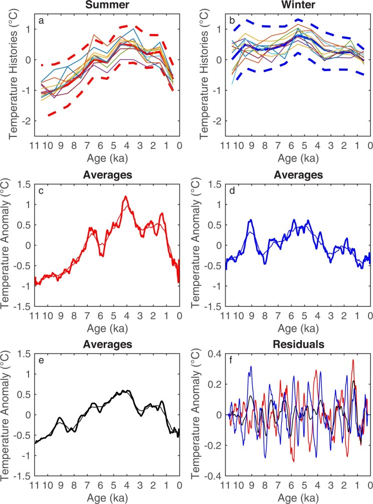
The recovery of long-term climate proxy records with seasonal resolution is rare because of natural smoothing processes, discontinuities and limitations in measurement resolution. Yet insolation forcing, a primary driver of multimillennial-scale climate change, acts through seasonal variations with direct impacts on seasonal climate¹. Whether the sensitivity of seasonal climate to insolation matches theoretical predictions has not been assessed over long timescales. Here, we analyse a continuous record of water-isotope ratios from the West Antarctic Ice Sheet Divide ice core to reveal summer and winter temperature changes through the last 11,000 years. Summer temperatures in West Antarctica increased through the early-to-mid-Holocene, reached a peak 4,100 years ago and then decreased to the present. Climate model simulations show that these variations primarily reflect changes in maximum summer insolation, confirming the general connection between seasonal insolation and warming and demonstrating the importance of insolation intensity rather than seasonally integrated insolation or season duration^2,3. Winter temperatures varied less overall, consistent with predictions from insolation forcing, but also fluctuated in the early Holocene, probably owing to changes in meridional heat transport. The magnitudes of summer and winter temperature changes constrain the lowering of the West Antarctic Ice Sheet surface since the early Holocene to less than 162 m and probably less than 58 m, consistent with geological constraints elsewhere in West Antarctica^4-7.

Fig. 1. Water-isotope seasonal variability.

a, Example section of the diffusion-corrected (solid line) and raw (dashed line) WDC δD records, with annual maxima (red circles) and minima (blue circles) determined algorithmically (Methods—Seasonal water-isotope amplitudes). Extended Data Fig. 1 provides the full high-resolution WDC δD record, diffusion lengths and extrema. b, The 50-yr annual-amplitude averages (summer minus winter divided by 2), with 2σ uncertainty; horizontal line indicates Holocene mean. c–e, The 50-yr δD averages for summer (red, c), mean (purple, d) and winter (blue, e); horizontal line indicates Holocene mean; shaded regions are 2σ bounds for combined analytical and diffusion-correction uncertainty. Source data

Fig. 2. Seasonal temperature reconstruction.

a,c, Reconstructed summer and winter temperatures at WDC for 1,000-yr averaging (solid red and blue lines). Shaded regions are 1σ and 2σ uncertainty ranges for combined uncertainties arising from analysis, diffusion correction, seasonality of accumulation, precipitation intermittency, isotope-temperature scaling and reconstructed mean temperatures (Methods—Uncertainties in reconstructing temperatures). Also shown are MEBM-calculated temperatures for 80° S (maximum and minimum annual values) and HadCM3 zonal temperatures for 80° S (late-December for summer, mid-August for winter) (ORBIT, GLAC1D and ICE-6G). The 0 ka ORBIT simulation uses pre-industrial settings, a calculation not available for GLAC1D or ICE-6G. Normalization is done at 1 ka when all model runs intersect within 0.05 °C and the ice-sheet configuration is well known. The ICE-6G values at 11 ka for summer and winter (not shown on plots) are −3.93 °C and −10.82 °C, respectively. Coefficient of determinations for model results versus WDC temperatures (Extended Data Fig. 7) are high for summer (HadCM3 ORBIT R² = 0.93, P ≪ 0.001; MEBM R² = 0.80, P ≪ 0.001) but not for winter (HadCM3 ORBIT R² = 0.00, P = 0.85; MEBM R² = 0.05, P = 0.30). The winter agreement improves if only the period 0–6 ka is considered (HadCM3 ORBIT R² = 0.74, P = 0.01; MEBM R² = 0.39, P = 0.02). b,d, Histograms of net temperature changes over the specified time intervals, derived by Monte Carlo analysis accounting for systematic and non-systematic uncertainties (Methods—Trend analysis). e, WDC mean annual temperature with 1σ and 2σ uncertainty bounds. Extended Data Table 2 shows the amount of variability in the mean annual temperature that can be explained by the summer and winter temperatures. Source data

Fig. 3. Temporal and spatial variability in insolation and model temperatures.

a, Insolation change through the Holocene for December and January and their average. December best resembles the WDC summer reconstruction. b, The full seasonal cycle of insolation at 80° S for 500-yr snapshots over the Holocene. Line colours in b and c correspond to age. c, Zoom of summer insolation. The maximum always occurs in the latter half of December (grey shading), migrating across 8 days over the course of the Holocene. d, Holocene trends of annual mean insolation (black), annual integrated insolation (dashed red line) and summer-integrated insolation (red line). e, Maximum summer insolation intensity (black line) and summer duration (red lines), defined as the number of days above a threshold insolation value each year. f, Anomaly in maximum insolation coloured by latitude in the Southern Hemisphere. The thick blue line shows the latitude of the WDC site. g, Calculated temperatures for 80° S using the MEBM, including maximum summer value (red), minimum winter value (blue) and amplitude of the seasonal temperature cycle (black). Source data

Fig. 4. Possible ice elevation histories and the corresponding modelled temperatures.

a, Elevation histories used in HadCM3. GLAC1D is 96 m higher at 11 ka compared to present and ICE-6G is 222 m higher. b, Temperature anomalies from elevation change (GLAC1D, solid lines; ICE-6G, dashed lines) using an atmospheric lapse rate of 9.8 °C km⁻¹ and spatial lapse rates for interior West Antarctica of 12 °C km⁻¹ (ref. ) and 14 °C km⁻¹ (ref. ). c, HadCM3 residual-temperature anomalies for December (summer) calculated by subtracting the ORBIT run from the GLAC1D and ICE-6G runs in Fig. 2a, highlighting the portion attributable to changing elevation rather than insolation. d, Residual-temperature change in b subtracted from the results in c, showing the component driven from processes besides the direct lapse-rate (LR) effect and orbital forcing. Source data

Extended Data Fig. 1. WDC water-isotope data.

a, The raw, high-resolution WDC δD water isotope record^– (grey), the raw 50-yr running mean (white), and the diffusion-corrected signal (black). b, The WDC diffusion-corrected δD record with extrema picks for summer (red) and winter (blue). c, The high-resolution diffusion length record (black; 140-yr windows, 70-yr time steps; 1σ uncertainty bounds in light grey) compared to prior estimates (red; 500-yr windows, 500-yr time steps). Source data

Extended Data Fig. 2. Precipitation uncertainties.

Uncertainties for seasonally weighted accumulation are shown in a-f, and for precipitation intermittency in g-h. a, The diffusion envelope of CFM output data (50-yr avg.), based on an input sine wave with f = 1yr⁻¹ and amplitude = 15.43‰. The original (input) amplitude of the signal (black, dotted-dashed lines) decreases as time passes due to diffusion and downward advection of the firn, as shown by the decay of the maximum (red) and minimum (blue) lines, while the mean values of the ‘constant’ and ‘cycle’ (black solid and dashed lines, respectively) scenarios do not change and are dependent on the seasonal weighting of snowfall. b, Diffused CFM output data from beneath the pore close-off depth (>200 yr) (black lines; smaller amplitude), with diffusion-corrected data shown with grey lines (larger amplitude). Red circles are the annual maximum value, and blue circles the annual minimum, selected using the same algorithm as Fig. 1a. c, A zoom of black carbon (BC) concentrations at ~6.5 ka^,. The maxima (red circles) and minima (blue circles) can be used to separate approximate depth intervals corresponding to winter (BC₁) and summer (BC₂); vertical blue lines correspond to nominal January 1, as defined by the peak of nssS/Na. d, The 140-yr averages for BC₁ (blue) and BC₂ (red). The grey line is WDC annual accumulation, orange circles are BC₁ + BC₂, which should equal annual accumulation. e, Black carbon seasonality BC₁/BC₂ (black), based on (d). f, Accumulation seasonality for HadCM3 seasonal snowfall (red line) compared to the range of seasonality tested using the CFM (dashed blue lines) and modern MAR seasonality (blue diamond). g, Distribution of annual amplitudes for water isotopes for a 1,000-year window centred at 4 ka. h, Standard errors are determined for 1,000-realizations of random sampling of the distribution in (g) to determine a standard deviation of the residuals of the true mean minus the mean of the random sampling.

Extended Data Fig. 3. Trend analysis.

a,b, The first 10 of 10,000 randomly generated, alternative seasonal temperature histories for summer (a) and winter (b), used in Fig. 2b,d to generate probability distributions of temperature trends in the Holocene. Thick, solid lines are mean values, and thick, dashed lines are 2σ uncertainty ranges. c–f, The 1,000-year (thin line) and 300-year (thick line) averages normalized to the 11-0 ka mean (c–e) and residuals (1,000 year minus 300 year) (f) of summer (red), winter (blue), and the mean (black), used to calculate R² values in Extended Data Table 2.

Extended Data Fig. 4. MEBM results.

MEBM seasonal surface temperatures are shown in a–c. a, Modelled seasonal surface temperature cycle at 80°S, coloured by age. b,c, Zoom in of modelled summer and winter temperature. MEBM annual results for the mean, maximum, and minimum are shown in d–l. Plots for temperature anomaly normalized to the mean (blue), insolation (red), and heat divergence (black) for the annual mean (d,g,j), annual max (e,h,k), and annual min (f,i,l). Note the sign of heat divergence; negative values correspond to heat convergence at the site.

Extended Data Fig. 5. 80°S energy balance at 10 ka.

Bar charts of HadCM3 energy balance terms at 10 ka for a, December (summer) and b, July (winter), including model runs for ‘orbit only’ (purple, ORBIT), ‘ice sheet only’ (blue, GLAC1D; green, ICE-6G), and ‘all forcings’ (orange, GLAC1D; yellow, ICE-6G). Positive values all indicate a surface or atmospheric warming. Variables include surface temperature (T_surf in °K), latent heat (LH in Wm⁻²), sensible heat to the surface (SH_d in Wm⁻²), shortwave radiation (SW in Wm⁻²), downward LW radiation (LW_d in Wm⁻²), and change in heat transport (∇·F in 10⁷ W).

Extended Data Fig. 6. Sea ice variability and temperature in HadCM3 simulations.

Maps of the dominant pattern of variability in each of the seasons and scatter plots of amplitude of the pattern against temperature. Maps were created using Python’s package cartopy. a,c, The EOF of sea ice variability in the Southern Hemisphere for December and July in ALL of the simulations: this is the dominant pattern of sea ice variability. b,d, The amplitude of the patterns in (a) and (c) vs. the temperature at 80°S for each simulation. Plots e–h show the zonal-mean temperature and sea ice in HadCM3 simulations for December average. e, Change in sea ice fraction for coupled-model simulations from 10 ka to 0 ka. f, Change in surface temperature between 10 ka and 0 ka for the coupled-model simulations (dotted line) and atmosphere-only simulations (solid line). g, Change in surface temperature for atmosphere-only runs from 10 ka to 0 ka. h, Change in surface temperature for atmosphere-only runs from 10 ka to 0 ka. See Extended Data Table 3 for descriptions of the model simulations used in panels (g) and (h).

Extended Data Fig. 7. Model results vs. WDC temperatures.

Coefficient of determination and p-values for comparison of HadCM3 (1-kyr resolution, n = 12) or MEBM (0.5-kyr resolution, n = 23) model results with WDC summer and winter temperatures.

References

1. Berger, A. Milankovitch theory and climate. Rev. Geophys.26, 624–657 (1988).
1. WAIS Divide Project Members. Onset of deglacial warming in West Antarctica driven by local orbital forcing. Nature500, 440–444 (2013). - PubMed
1. Huybers, P. & Denton, G. Antarctic temperature at orbital timescales controlled by local summer duration. Nat. Geosci.1, 787–792 (2008).
1. Ackert, R. P. et al. Measurements of past ice sheet elevations in interior West Antarctica. Science286, 276–280 (1999). - PubMed
1. Steig, E. J. et al. in The West Antarctic Ice Sheet: Behavior and Environment Vol. 77 (eds Alley, R. B. & Bindschadle, R. A.) 75–90 (American Geophysical Union, 2001).
Publication types