Concentration-Dependent Domain Evolution in Reaction-Diffusion Systems

Abstract

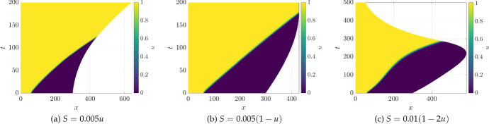
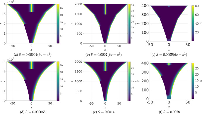
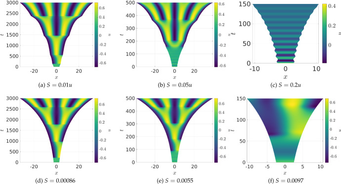
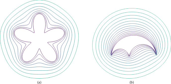
Pattern formation has been extensively studied in the context of evolving (time-dependent) domains in recent years, with domain growth implicated in ameliorating problems of pattern robustness and selection, in addition to more realistic modelling in developmental biology. Most work to date has considered prescribed domains evolving as given functions of time, but not the scenario of concentration-dependent dynamics, which is also highly relevant in a developmental setting. Here, we study such concentration-dependent domain evolution for reaction-diffusion systems to elucidate fundamental aspects of these more complex models. We pose a general form of one-dimensional domain evolution and extend this to N-dimensional manifolds under mild constitutive assumptions in lieu of developing a full tissue-mechanical model. In the 1D case, we are able to extend linear stability analysis around homogeneous equilibria, though this is of limited utility in understanding complex pattern dynamics in fast growth regimes. We numerically demonstrate a variety of dynamical behaviours in 1D and 2D planar geometries, giving rise to several new phenomena, especially near regimes of critical bifurcation boundaries such as peak-splitting instabilities. For sufficiently fast growth and contraction, concentration-dependence can have an enormous impact on the nonlinear dynamics of the system both qualitatively and quantitatively. We highlight crucial differences between 1D evolution and higher-dimensional models, explaining obstructions for linear analysis and underscoring the importance of careful constitutive choices in defining domain evolution in higher dimensions. We raise important questions in the modelling and analysis of biological systems, in addition to numerous mathematical questions that appear tractable in the one-dimensional setting, but are vastly more difficult for higher-dimensional models.

Keywords: Evolving domains; Linear instability analysis; Pattern formation.

Fig. 1

(Color Figure Online) Values of u from 1D simulations of the logistic kinetics (26) under different growth scenarios. In all simulations, the initial domain length is $L=30$, with $D_1=1$. The initial condition is taken as $u(0,x)=(1+tanh(L/5-x))/2$, so that the leftmost $20\%$ of the domain has the initial value $u\approx 1$ and the rest has the value $u\approx 0$

Fig. 2

(Color Figure Online) Values of u from 1D simulations of the Schnakenberg kinetics (23) under different growth scenarios. In all simulations the initial domain length is $L=5$, with $a=0.01$, $b=1.1$, $D_1=1$, and $D_2=40$. In (d)–(i), we show u-dependent growth, whereas in (a)–(c) we show uniform exponential domain growth. Timescales are set so that all domains grew to $\approx 670$. Uniform growth rates were used in (a)–(c) to match the corresponding domain lengths and timescales in (d)–(f), so that the final simulation time and domain sizes are identical

Fig. 3

(Color Figure Online) Values of u as black curves and S as green curves at specific times from the same simulations in Fig. 2. Row (a)–(c) corresponds to panel (a) in Fig. 2, Row (d)–(f) corresponds to panel (c) in Fig. 2, row (g)–(i) corresponds to panel (f) in Fig. 2, and Row (j)–(l) corresponds to panel (i) in Fig. 2. The first column is taken at 1/3 of the final simulation time, the second at 2/3 of the final simulation time, and the last column at the final simulation time

Fig. 4

(Color Figure Online) Values of u from 1D simulations of the Schnakenberg kinetics (23) under different growth scenarios. In all simulations, the initial domain length is $L=10$, except in (f) where $L=5$, with $a=0.01$, $b=1.1$, $D_1=1$, and $D_2=40$

Fig. 5

(Color Figure Online) Values of u from 1D simulations of the Gierer–Meinhardt kinetics (24) under different growth scenarios. In all simulations the initial domain length is $L=10$, with $a=0.01$, $b=0.5$, $c=5.5$, $D_1=1$ and $D_2=200$. The timescale and growth rates in (a)–(c) are chosen to match those in (e)–(g) so that the final simulation time is on a domain of exactly the same size

Fig. 6

(Color Figure Online) Values of u from 1D simulations of the FitzHugh–Nagumo kinetics (25) under different growth scenarios. In all simulations the initial domain length is $L=5$, with $a=1.01$, $b=1$, $c=1$, $i_0=1$, $D_1=1$ and $D_2=2.5$. The timescale and growth rates in (a)-(c) are chosen to match those in (d)-(f), so that the final simulation time is on a domain of exactly the same size

Fig. 7

(Color Figure Online) Two examples of the growth of a boundary with the locally uniform expansion rate $S=0.001$. In (a) we start with a starfish-like domain given by equation (13) in Krause et al. (2021) for $\gamma =0.8$ and $L=1$. In (b) we start with an Arbelos-like domain composed of the boundaries of three semicircles of radius 1, 2/5, and 3/5, respectively, with some truncation done near the lower boundary to prevent issues with extremely small finite elements. Boundary curves shown are arranged so that larger enclosed areas correspond to later times, with times uniformly sampled

Fig. 8

(Color Figure Online) Values of u from 2D simulations of the scalar bistable kinetics (27) in the dumbbell-shaped domain given by (29) with the diffusion parameter $D=1$ and growth rate $S=0.000125(1+tanh(50(u-0.9))$. Iterations are shown at times $t=0,8,2392,3192,4792,$ and 5272

Fig. 9

(Color Figure Online) Plots of the domain boundary from 2D simulations of the scalar bistable kinetics (27) in the dumbbell-shaped domain given by (29) with the diffusion parameter $D=1$. Panel (a) corresponds to Fig. 8 with $S=0.000125(1+tanh(50(u-0.9))$, and panel (b) to a simulation with $S=0.000125(1+tanh(50(|u|-0.9))$. Boundary curves shown are arranged so that larger enclosed areas correspond to later times, with times uniformly sampled

Fig. 10

(Color Figure Online) Values of u from 2D simulations of the Gierer–Meinhardt kinetics (24) in an initially circular domain of radius 3. The parameters used are $D_1=1$, $D_2=1000$, $a=0.01$, $b=0.5$, $c=5.5$, with a growth rate of $S=0.001(1+tanh(100(u-22))$. Iterations are shown at equally spaced times with all panels using the same spatial scale

Fig. 11

(Color Figure Online) Values of u from 2D simulations of the Gierer–Meinhardt kinetics (24) in an initially circular domain of radius 3. The parameters used are $D_1=1$, $D_2=1000$, $a=0.01$, $b=0.5$, $c=5.5$, with a growth rate of $S=0.001({(u/u^{\ast })}^2-1)=0.001({(u/11.02)}^2-1)$. Iterations are shown at equally spaced times, with panels (d) and (e) being the same plot but resized so that panels (a)-(d) are shown on the same scale and panels (e)-(h) are shown on the same scale

Fig. 12

(Color Figure Online) Plots of the domain boundary from 2D simulations of the Gierer–Meinhardt kinetics (24). Panel (a) corresponds to Fig. 10 and panel (b) to Fig. 11. Boundary curves shown are arranged so that larger enclosed areas correspond to later times, with times uniformly sampled. In panel (b), later boundary curves are to the left but do not enclose larger areas due to contraction towards the right side of the domain

References

1. Adamer MF, Harrington HA, Gaffney EA, Woolley TE. Coloured noise from stochastic inflows in reaction-diffusion systems. Bull Math Biol. 2020;82(4):1–28. - PMC - PubMed
1. Baker RE, Maini PK. A mechanism for morphogen-controlled domain growth. J Math Biol. 2007;54(5):597–622. - PubMed
1. Bao W, Yihong D, Lin Z, Zhu H. Free boundary models for mosquito range movement driven by climate warming. J Math Biol. 2018;76(4):841–875. - PubMed
1. Barreira R, Elliott CM, Madzvamuse A. The surface finite element method for pattern formation on evolving biological surfaces. J Math Biol. 2011;63(6):1095–1119. - PubMed
1. Batchelor GK (1967) An introduction to fluid dynamics. CUP
Publication types
LinkOut - more resources