Spontaneous behaviour is structured by reinforcement without explicit reward

Abstract

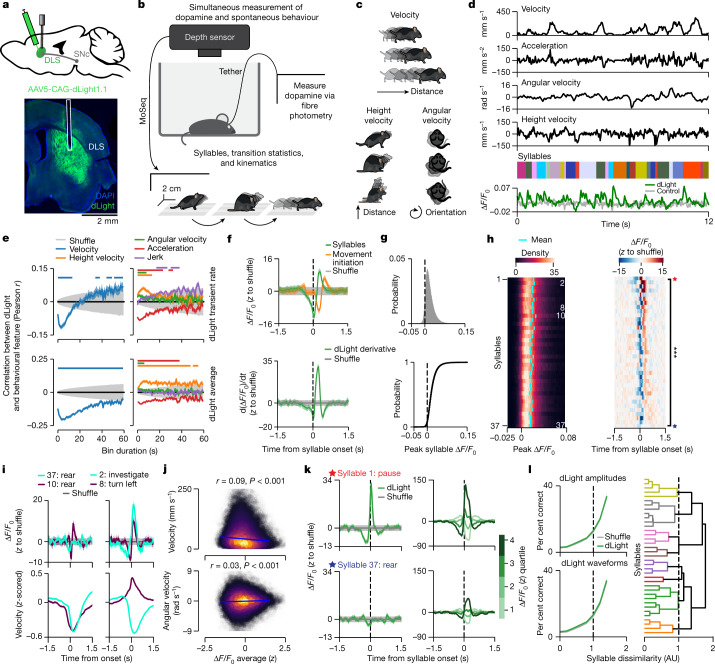
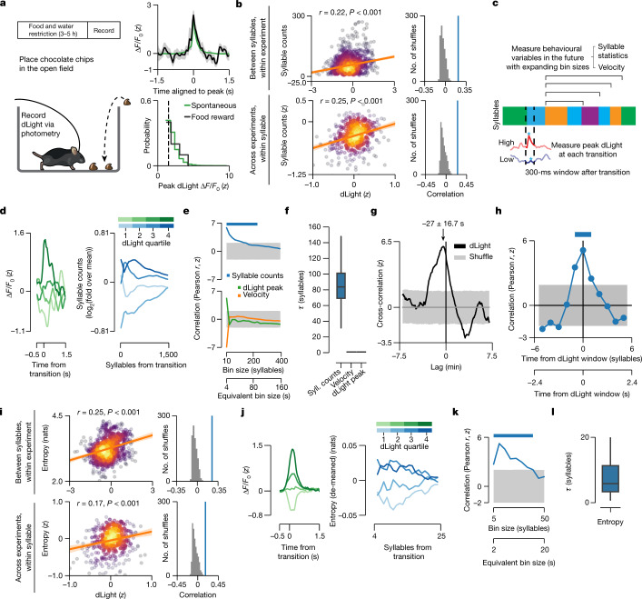
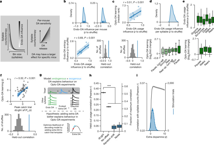
Spontaneous animal behaviour is built from action modules that are concatenated by the brain into sequences^1,2. However, the neural mechanisms that guide the composition of naturalistic, self-motivated behaviour remain unknown. Here we show that dopamine systematically fluctuates in the dorsolateral striatum (DLS) as mice spontaneously express sub-second behavioural modules, despite the absence of task structure, sensory cues or exogenous reward. Photometric recordings and calibrated closed-loop optogenetic manipulations during open field behaviour demonstrate that DLS dopamine fluctuations increase sequence variation over seconds, reinforce the use of associated behavioural modules over minutes, and modulate the vigour with which modules are expressed, without directly influencing movement initiation or moment-to-moment kinematics. Although the reinforcing effects of optogenetic DLS dopamine manipulations vary across behavioural modules and individual mice, these differences are well predicted by observed variation in the relationships between endogenous dopamine and module use. Consistent with the possibility that DLS dopamine fluctuations act as a teaching signal, mice build sequences during exploration as if to maximize dopamine. Together, these findings suggest a model in which the same circuits and computations that govern action choices in structured tasks have a key role in sculpting the content of unconstrained, high-dimensional, spontaneous behaviour.

Fig. 1. Behaviour is associated with dopamine transients in DLS.

a, dLight expression and fibre placement in DLS (Methods). b, The behavioural characterization pipeline using MoSeq (n = 14 mice for MoSeq, 216 experiments; Methods). c, Examples of measured kinematic variables. d, Aligned kinematic variables, MoSeq syllables and dLight fluorescence from an example experiment. e, Top, average correlation between kinematic variables and dLight transient rate. Bottom, correlations with dLight fluorescence. Coloured shading denotes bootstrapped s.e.m.; grey shading indicates the 95% shuffle confidence interval. Solid bars indicate statistical significance at P < 0.05 (shuffle test; Methods). f, Top, average fluorescence (z-scored to shuffle; Extended Data Fig. 4c and Methods) aligned to movement initiation or syllable onsets (n = 100 shuffles). The average syllable-associated dLight transient exceeds that associated with movement initiation (P = 0.0006, z = 3, effect size r = 0.8, two-sided Wilcoxon signed-rank test; n = 14 averages). Bottom, derivative of top panel. Green shading represents the 95% bootstrap confidence interval; grey shading represents the 95% shuffle confidence interval. g, The distribution of all syllable-associated dLight peaks. Bottom, the cumulative distribution. h, Left, the distribution of syllable-associated dLight peaks for across all experiments. Right, z-scored average syllable-associated waveforms, sorted by peak fluorescence. The blue and red stars indicate the syllable waveforms shown in k. ***, Kruskal–Wallis H test on average syllable-associated fluorescence amplitudes: P < 10⁻²⁵, H = 209.29, n = 518 mouse–syllable pairs. y-axis syllable sorting is shared across panels. i, Left, example syllables with different average (across experiments) waveforms (top) but similar velocity (bottom). Right, example syllables with similar waveforms (top) but different velocities (bottom). Shading represents the 95% confidence interval. j, Robust linear regression between syllable-associated dLight and velocity (top) or angular velocity (bottom; Methods). Each point is a sampled syllable instance (n = 28,000 points; n = 2,000 points per syllable drawn randomly from each mouse). Regression line (shading indicates the 95% bootstrap confidence interval) and kernel density estimate are shown. P-values estimated by shuffle test. k, Left, average syllable-associated waveforms for starred syllables in h (right). Coloured shading represents the 95% bootstrap confidence interval; grey shading represents the 95% shuffle confidence interval. Right, syllable-associated waveforms from the left panel binned into quartiles of peak magnitudes. l, Left, held-out classifier performance predicting syllable identity from syllable-associated dLight peak amplitudes (top) or waveforms (bottom). Right, dendrogram showing syllables organized by MoSeq distance (Methods). AU, arbitrary units.

Fig. 2. Endogenous dopamine transients predict average syllable use and sequence variability.

a, The unexpected food reward protocol. Top right, average spontaneous versus food reward-associated transients (Methods). Shading represents bootstrap s.e.m. Bottom right, probability density function of dLight transient amplitudes. The dotted line indicates the threshold for detecting dLight transient peaks. b, Left, robust linear regression between syllable-associated dLight and average syllable counts per syllable (each dot is a syllable–mouse pair). Regression line and kernel density estimate are shown (r is Pearson correlation between held-out predictions and actual data). Right, the distribution of Pearson correlations using models fit to shuffled data compared with the observed correlation (blue line). Shading indicates the 95% bootstrap confidence interval. P-values estimated by one-sided shuffle test. c, Schematic depicting the hypothesis that dopamine predicts changes in future behaviour. Blue star indicates the syllable-associated dopamine peak. d, Left, average dLight waveforms for each fluorescence quartile at syllable onset for an example syllable–experiment pair. Right, log₂ fold change compared to average syllable counts after example syllable onset computed over increasing bin sizes (in syllables) after onset. e, The average Pearson correlation between syllable-associated dLight and syllable counts or velocity, and the dLight signal autocorrelation, computed using a set of increasing bin sizes after syllable onset. Grey shading represents the shuffled 95% confidence interval. The two x-axes reflect time in syllables and approximated in seconds. Solid bars indicate statistical significance (P < 0.05, one-sided shuffle test). f, The distributions of exponential decay timescales (τ) for the correlations plotted in Fig. 2e (n = 1,000 bootstrap samples). In all box plots in this Article, the horizontal line represents the median, box edges delineate the first and third quartiles, and whiskers include the furthest data point within 1.5 times the interquartile range of the first or third quartile. g, Average cross-correlation between binned syllable counts and syllable-associated dLight fluorescence (from all mice and experiments) across lags (P < 0.001, one-sided shuffle test; the arrow indicates average peak lag, error is 68% confidence interval). Grey shading represents the shuffled 95% confidence interval. h, Overall correlation between syllable-associated dLight and syllable usage for syllables temporally adjacent to the index syllable. Grey shading represents the shuffled 95% confidence interval. The solid bar denotes statistical significance (P < 0.05, one-sided shuffle test). i, As in b, but for average entropy per syllable. Nat, natural unit of information. j, As in d, but for sequence entropy for an example syllable–experiment pair. k, As in e, but for sequence entropy. l, Fitted τ values for the correlation curve in k (n = 1,000 bootstrap samples).

Fig. 3. Optogenetically evoked dopamine release in DLS reinforces syllable use and increases sequence variability.

a, The closed-loop MoSeq pipeline. b, Schematic and representative brain section of fibre cannulae over DLS dopamine axons. c, Top, normalized optogenetically evoked dLight peak magnitude distribution (n = 842 peaks). Bottom, mean waveforms from spontaneous and Opto-DA transients (Methods). Shading represents the 95% bootstrapped confidence interval. Max, maximum. d, Experimental schedule describing baseline (rec.) and stimulation (stim.) sessions for ‘target’ syllables (Methods). e, log₂ fold change in target counts compared with baseline, per mouse, averaged across targets (P = 0.002, U = 197, f = 0.82, one-sided Mann–Whitney U test) (see Methods for definition of ‘learner’). f, Cumulative increase in target counts relative to baseline in Opto-DA and control mice (P = 0.007, U = 184, f = 0.77, one-sided Mann–Whitney U test). g, Cumulative counts over concatenated stimulation sessions per target. Shading indicates bootstrap s.e.m. h, The relationship between target syllable usage changes from baseline during stimulation experiments versus post-stimulation experiments per mouse (Pearson r = 0.89, P = 0.005 for learners and P = 0.082 for controls, one-sided shuffle test). NS, not significant. i, Average transition entropy following stimulation. Shading indicates bootstrap s.e.m. The light grey band indicates the 95% confidence interval of the pre-stimulation average. Data are binned using five-syllable-wide non-overlapping bins. The bar indicates significance (P < 0.05 for Opto-DA mice, P > 0.05 for controls, two-sided Mann–Whitney U test comparing stimulation with catch trials). Syll, syllable. j, Sequence context changes from baseline to post-stimulation for an example mouse–target pair. Sequences proceed from left (incoming syllables) to right (outgoing syllables). Nodes are sorted by decreasing frequency at baseline. k, Average change in inbound and outbound transitions for target syllables on stimulation day sorted by the baseline rank of the transition. Traces are smoothed with a five-point rolling average. Shading indicates bootstrap s.e.m. l, Average kinematic parameters aligned to stimulation in Opto-DA mice and controls. Shading as in i. No comparisons between stimulation and catch trials in any of the mice were significant (P > 0.05, one-sided Mann–Whitney U test). m, As in l, but following 3-s-long stimulation. The solid bar indicates significance (P < 0.05, one-sided Mann–Whitney U test).

Fig. 4. Optogenetic syllable reinforcement varies predictably across mice and syllables.

a, Schematic depicting the relationship between observed endogenous dopamine-syllable usage correlations and per-mouse dopamine sensitivity. Dopamine (DA) sensitivity refers to the ability of endogenous, syllable-associated dopamine peaks to influence changes in syllable counts (Endo-DA count influence) or sequencing (Endo-DA entropy influence) within an experiment (see Methods for how indices were computed). b, Top, the distribution of per mouse Endo-DA count influence (left) and Endo-DA entropy influence (right) averaged across all syllables. Bottom, scatter plot (including linear regression model fit) of per mouse average Endo-DA count influence and Endo-DA entropy influence (Pearson r = 0.69 computed from model predictions on leave-two-out held-out data; P = 0.001, P-value computed via one-sided shuffle test). Shading indicates the 95% bootstrap confidence interval. c, Scatter plot (including regression line) of per mouse average Opto-DA learning versus Endo-DA count influence (Pearson r = 0.51 (computed from model predictions on leave-two-out held-out data); P = 0.001, P-value computed via one-sided shuffle test). Shading indicates the 95% bootstrap confidence interval. d, Top, the distribution of per syllable average Endo-DA count influence (n = 296 mouse–syllable pairs). Bottom, Opto-DA learning plotted syllable-by-syllable for ‘learner’ mice (n = 9 mice). e, Top, average Endo-DA count influence across syllable categories. Bottom, average Opto-DA learning across syllable categories. f, Top, scatter plot (including regression line) of catch trial syllable-associated dLight and Opto-DA learning for each mouse–syllable pair (r = 0.32 over held-out data; P < 0.001, estimated via one-sided shuffle test). Bottom, model performance (evaluated with five times fivefold cross-validation) using actual versus shuffled data. g, Hypothesis that evoked dopamine release combines with ongoing endogenous release to alter behavioural choices. h, Model-based likelihood of predicting held-out syllable choices on Opto-DA stim experiments (blue) relative to control models (Methods) (P = 7 × 10⁻¹⁸ across all model comparisons relative to dLight model, U = 2,500, f = 1, two-sided Mann–Whitney U test; n = 50 model restarts; Methods). The right y-axis indicates the model performance as a fraction the of maximum correlation. i, The relationship between average model accuracy (correlation between predicted syllable usage and actual usage) and the ‘extra dopamine’ free parameter (black). Shading indicates the 95% bootstrap confidence interval. The distribution of empirically measured optically evoked dLight fluorescence is shown in blue.

Fig. 5. RL models suggest that mice attempt to maximize dopamine during spontaneous behaviour.

a, Top, schematic describing modification of a standard RL model to explore relationships between DLS dopamine fluctuations and behavioural choices. Bottom, schematics of ‘reinforcement-only’ and ‘full’ model variants (Methods). b, Left, empirical transition matrix (TM) observed during open field behaviour. Centre, an example transition matrix learned by the full model (top), along with the squared difference between the empirically observed transition matrix and the example learned transition matrix (bottom). Right, as in centre, except for the reinforcement-only model. The average correlation between the observed transition matrix and the transition matrix learned by each model, along with the associated P-value computed via shuffle test, are given for each model type. For visualization, the model transition matrix is estimated by taking a softmax (see Methods) over the Q-table learned by the model. Here, the temperature parameter was set to 0.1 for visualization only. c, The distribution of correlations between the learned and observed transition matrices for both the reinforcement-only (blue) and full (orange) models, compared to a histogram of correlations between transition matrices learned with time-shuffled dLight traces (all models are statistically significant according to a shuffle test, defined as model fits exceeding 95% of shuffle correlation values, n = 100 shuffles). d, The performance of the full model after temporally shifting syllable-associated dLight amplitudes across syllables over various lags. e, The distribution of log likelihoods for models that consider dopamine as a reward versus a reward-prediction error (RPE) signal (Methods). The log likelihoods shown are for the best parameterization for each model type across 50 bootstraps of the dataset. On the basis of this relationship, we formulated models that treated dopamine transients as representing reward rather than reward-prediction error.

Extended Data Fig. 1. dLight validation, photometry setup and motion artifact removal.

a) Maximum projection epifluorescence images of HEK cells transfected with the dLight plasmid, and excited with either 480 nm blue (top) or 400 nm UV (bottom) light. Green emission (527 nm) was collected for both excitation wavelengths. Scale bar indicates 20 µm. Three separate experiments were performed with n = 28, n = 45, n = 42 regions of interest (ROIs) from the first, second, and third experiment respectively. b) Scatter plot of pixel fluorescence for each pixel location under both 400 nm and 480 nm excitation. A regression line was fit to the scatter plot (blue). The strength of the correlation demonstrates that both excitation wavelengths cause similar spatial patterns of dLight emission at 527 nm. c) Single cell dLight responses to perfused dopamine at 480 nm (left) or 400 nm (right) wavelengths. White dashed lines indicate time points where dopamine is washed into and out of the sample. Each row is an individual cell region of interest (ROI). d) Correlation in single cell dLight responses to perfused dopamine imaged with blue (x-axis) or UV light (y-axis). Each dot is an individual cell. Blue line indicates linear fit. The near-zero slope indicates that the UV-light-dependent green emission is almost entirely independent of dopamine concentration. e) Validation of dLight1.1 response to optogenetic stimulation. To assess how quickly DLS dLight reports dopamine transients in vivo, SNc axons were optogenetically stimulated using ChrimsonR (whose excitation spectrum is separated from that of dLight) while dLight fluorescence was recorded. Left: schematic illustrating viral injection and implant procedure to simultaneously record dLight transients and optogenetically stimulate dopamine axons in DAT-Cre animals. dLight was injected into the right dorsolateral striatum, Cre-dependent ChrimsonR was injected into the right SNc, and an optical fiber was placed above the dLight injection site in the DLS (see Methods). Middle: coronal slice depicting the expression of both dLight and ChrimsonR in the striatum. Right: mean stimulation-evoked dLight fluorescence using ChrimsonR in dopaminergic axons originating from SNc. The green shaded region indicates bootstrap SEM. The gray shaded area indicates the 95% bootstrap confidence interval of the mean trace pre-stimulation. Red shading indicates the duration of optogenetic stimulation. dLight transients are resolvable starting 67 ms from stimulation onset, suggesting that dLight can report rapid dopamine dynamics via photometry in DLS (p = 0.005, U = 2610, f = 0.32, one-sided Mann-Whitney U test). f) Schematic describing the photometry recording setup. A blue and UV LED were modulated at different frequencies, and light delivered to the mouse via a single fiber optic cable. Green fluorescence was acquired using a photodetector and the blue (dLight) and UV (isosbestic) components were separated using lock-in amplification. g) Example data depicting a dLight trace along with the simultaneously recorded reference signal acquired during free behaviour. The UV, or reference signal, represents the contributions of motion and mechanical artifacts and other non-ligand dependent changes in sensor fluorescence. Since UV and blue excitation of dLight cannot be perfectly matched, a gain and bias term were fit to match the UV-excited emission to the blue-excited emission per previously published papers; this fitting process maximizes the correlation between the UV and blue signals, enabling us to effectively subtract the reference signal from the dLight signal. Left: example fit showing the UV trace scaled to match the dLight trace (bottom) aligned to syllables (top). Right: histogram of r² values between the photometry reference (UV component) and signal (dLight component), prior to fitting and subtracting the reference signal (top) and after fitting and subtracting the reference signal (bottom). Note that the baseline correlation between the reference and signal channels prior to subtraction is low. h) Top: the probability, on average, of observing a dopamine transient across all mice and experiments – defined as the ΔF/F0 trace crossing 1 standard deviation (computed per experiment) – at a given timepoint in the experiment. The probability was estimated in one minute bins. Shading indicates the 95% bootstrap confidence interval across per-mouse averages. Bottom: the maximum ΔF/F0 per 1 min time bin across all mice and experiments. As in the top plot, the average across all mice and experiments is shown, with shading indicating the 95% bootstrap confidence interval across per-mouse averages.

Extended Data Fig. 2. MoSeq captures subsecond structure in spontaneous mouse behaviour.

a) Distribution of syllable durations identified by MoSeq. The mean/median syllable duration was 566/400 ms +/− 636 ms SD. b) The average number of times each MoSeq-identified syllable is used during a 30-minute experiment per mouse (n = 16 mice). Error bars indicate bootstrap 95% confidence intervals across mice. c) Human-annotated descriptions of observed behavioural syllables. Left: semantic labels and “spinograms” of all behavioural syllables used more than 1% of the time, here to provide an illustration of movements associated with syllables. Each trace in the spinogram is an average height profile of the mouse computed by taking the pixel values along the center of the depth image across columns (note that MoSeq pre-processes depth images so that mice always face to the right of the cropped depth image). Each trace from left to right is the average of each frame of the behavioural syllable from the beginning to end. The distances between successive traces are proportional to the average x/y displacement from one frame to the next. Spinograms are color-coded by the average angular velocity of the syllable. Right: dendrogram computed using the pairwise MoSeq distance of all behavioural syllables (see Methods for a description of how MoSeq distances, which capture the average three-dimensional pose dynamics of each syllable, are computed). Spinograms are aligned to their corresponding leaf in the dendrogram. d) The average transition matrix visualized as a state map. Each circle corresponds to a syllable, and each arrow corresponds to the likelihood that there is a transition from one syllable to the next. Arrow width indicates transition probability. All transitions with a probability below 0.1 are removed for visual clarity in this statemap and in all subsequent statemaps. e) Kinematic parameters over time averaged across all experiments and mice, demonstrating non-stationarities in kinematics across each recording experiment. Lines indicate boundaries derived via k-means clustering of this data. Note that these boundaries were used for analysis shown in Fig. 2e and k. Specifically, in order to prevent non-stationarities from impacting within-experiment correlations, correlations were computed within each of these segments and then averaged. f) Heatmap of syllable counts computed over a six-minute sliding window for the 37 syllables used >1% of the time in an example experiment. Syllables are sorted by total usage in the experiment, with the most-used syllable at the top and least used on the bottom. The colors above each segment of the plot indicate the time intervals used to compute the transition matrices in Extended Data Fig. 2g. g) State maps computed for each colored section of the example experiment shown in Extended Data Fig. 2f, summarizing the transition statistics between behavioural syllables, and demonstrating that transitions are also non-stationary over each imaging experiment. Each node is a syllable, and each line represents the transition from one syllable to the next (whose width specifies the observed likelihood of each transition, per the legend).

Extended Data Fig. 3. Validating correlations to kinematic variables through multi-camera keypoint tracking.

a) 15 keypoints were tracked in 3D using 6 infrared cameras (Azure Kinect, see Methods) positioned around the open field arena (n = 5 mice). A custom keypoint detection network was trained to identify all keypoints using manually labeled frames from each individual camera and integrated post-hoc with GIMBAL (see Methods). Top: schematic of keypoints positioned on the mouse. Bottom: example aligned frames from each of the 6 cameras with keypoints superimposed. b) Pearson correlation between 2D velocity and simultaneously recorded dLight at different timescales. 2D velocity was estimated by computing the centroid of the spinal keypoints in the X and Y plane for each frame (shown as the dark blue keypoints in Extended Data Fig. 3a) and taking the difference between centroid positions across frames. As in Fig. 1e, 2D velocity is negatively correlated with dLight transient rates at short timescales, and positively correlated at long timescales. Top: Pearson correlations between 2D velocity and dLight transient rates across various time bins. Bottom: Pearson correlations between 2D velocity and average dLight fluorescence across various time bins. Shading represents 68% CI. c) Left: correlation between 2D velocity and dLight fluorescence after binning the data into 400ms time points (Pearson r = −0.16, p < .001 one-sided shuffle test). Each dot is a single 400ms time bin. Color represents point density, where brighter colors indicate denser points. Right: correlation between 3D forelimb velocity and dLight fluorescence after partialing out the relationship between dLight and other known kinematic parameters such as velocity and height (see Methods, Pearson r = −0.02, p < .001 one-sided shuffle test).

Extended Data Fig. 4. Variability of syllable-specific dLight waveforms across mice and experiments.

a) Average dLight fluorescence aligned to syllable onset after time warping (traces were warped using linear interpolation from syllable onset to syllable offset, see Methods). b) Average probability of a syllable transition occurring near a dLight peak across all experiments. Peaks in the dLight trace were identified by first computing and z-scoring the derivative of the ΔF/F0 trace, and identifying peaks as values that exceeded the 90^th (left), 95^th (middle), or 99^th (right) percentile. We then plotted the probability that a syllable transition occurred given a dopamine peak. Gray shading indicates 95% bootstrap confidence interval of the shuffle. For the 95^th percentile threshold, a syllable transition is likeliest to occur 200 ms prior to the dLight peak. However, the estimated dLight peak lags actual dopamine release by 10s of milliseconds (Extended Data Fig. 1e). c) Left: schematic showing forms of variability in dLight fluorescence measurements across experiments. dLight fluorescence assessed via photometry often exhibits baseline shifts and shifts in fluorescence scaling that can be normalized across experiments by z-scoring the fluorescence trace. Z-scoring dLight per experiment will have the effect of shifting the distribution leftward (and thus producing negative values). Top right: distribution of all syllable-associated dLight peaks across all mice and all experiments (left), and corresponding cumulative distribution (right). Bottom right: distribution of all syllable-associated dLight peaks across all mice and all experiments after z-scoring fluorescence traces from each experiment (left), and corresponding cumulative distribution (right). d) Left: assessing variability of the average dLight transient amplitudes from mouse to mouse. Shown is the average dLight amplitude aligned to syllable transitions Z-scored relative to a shuffle as in Fig. 1f. The thick black line indicates the average across all mice, and per-mouse averages are shown as thin gray lines. Right: same as left except averages across experiments are shown; the thick black line indicates the overall average, and the thin gray lines are per-experiment averages. e) Pseudo-color plots where each row depicts per-experiment average aligned to syllable onset for all experiments, grouped by mouse. Gray lines indicate boundaries between individual mice. f) Left: pseudo-color plot of all per-syllable dLight waveforms as in Fig. 1h, except shown for each mouse. The color bar on the left indicates which rows correspond to which syllables using the same sorting as Fig. 1h. Within a syllable-specific block, individual rows correspond to per-mouse average dLight waveforms (n = 518 syllable/mouse pairs). Average dLight waveforms are z-scored to a shuffle. Right: the syllable-associated peak dLight value for each row, computed from each waveform between 0–300 ms from syllable onset. g) Average dLight fluorescence aligned to syllable onset for three example syllables shown in Extended Data Fig. 4e; the thick black line indicates the mean across all experiments, with the thin grey lines indicating averages from each mouse. h) The probability of observing a syllable-specific dLight peak value across every syllable instance and across all mice and experiments. Syllable-specific peak values are computed using the maximum value in a 300 ms window after syllable onset. Here, color values indicate the likelihood of observing a specific peak dLight amplitude from trial to trial without averaging. Here, dLight is z-scored within each experiment. Cyan bars show the location of the overall average for each syllable. Rows are sorted in the same order as Fig. 1h and Extended Data Fig. 4f. i) The probability of syllable-specific average dLight peak values across experiments. Syllable-specific peak values are computed using the maximum value in a 300 ms window after syllable onset and averaged over the experiment, and thus do not correspond to the average waveform peaks in Extended Data Fig. 4e. Each row corresponds to a given syllable, and color values indicate the likelihood of observing a given peak dLight amplitude, on average, across experiments. Here, average dLight peaks are z-scored within each experiment. Cyan bars show the location of the overall average for each syllable. Rows are sorted in the same order as Fig. 1h and Extended Data Fig. 4f.

Extended Data Fig. 5. Querying different possible sources of variability in dLight waveforms.

a) Average per-syllable dLight peaks associated with six behavioural categories (n = 7 dive syllables, 7 grooms, 9 pauses, 13 rears, 5 scrunches, 16 walks). Each category is associated with multiple syllables and were identified through human annotation. b) Within-syllable changes in kinematic parameters do not covary with peak dLight. Box plots of kinematic parameters binned by syllable-associated peak dLight – shown are the first and fourth quartiles. Kinematic variables were averaged from syllable onset to syllable offset, and box plots show the distribution of per-instance averages. Box plots for two examples syllables are shown, an investigatory pause (top; N = 15245 syllable instances) and a scrunch (bottom; N = 11838 syllable instances). c) Left top: average dLight fluorescence waveforms for two syllables that contain a left- (contralateral) and right-ward (ipsilateral) turning component. Consistent with prior studies indicating that elevated dopamine and striatal activity is associated with contralateral turning, we find higher average dLight levels are associated with contralateral turning^,. Fluorescence traces were z-scored to a circular shuffle. Left bottom: dLight waveforms broken out into quartiles based on syllable-associated fluorescence, as in Fig. 1k. Right: performance of a linear SVM classifier predicting individual syllable instances as left or right turns. Average observed accuracy was 51%, indicating substantial instance-by-instance variability (p < .001, one-sided shuffle test). d) Schematic illustrating the hypothesis that dopamine fluctuations may reflect performance prediction errors; here “performance error” is defined as the degree to which a given syllable instance differs from its mean implementation (see Methods). e) Top: schematic describing the linear model used to characterize whether syllable rendition quality compared to a template provides additional information about dLight fluorescence on top of the kinematic parameters described in Fig. 1e. Bottom: model coefficient for each kinematic parameter. Significant parameters are shaded black (p < .001 two-sided shuffle test, n = 1000 bootstraps; error bars indicate 95% CI). f) Left half: Distribution of dLight waveforms across different velocity change bins. Syllable transitions were binned by the change in velocity from one syllable to the next. The peak magnitudes of dLight waveforms within each “velocity change” bin were then binned from lowest to highest; these binned dLight waveforms reveal the diversity of dLight transients associated with each behavioural transition type. Left: averaged velocity traces for each velocity change/dLight peak bin pair. Right: averaged dLight traces for each velocity change/dLight peak bin pair. Right half: Same as left half, but transitions were binned by their associated jerk, and waveform distributions are plotted as described above. Here inter-syllable jerk is used as a surrogate for the biomechanical difficulty mice are likely to experience as they transition across syllables. g) Syllable-associated dopamine peaks do not contain information about position in the open field. For each syllable, peak dLight and velocity were binned into ten equally spaced bins, and the animal’s 2D centroid position in the arena was binned into four equally spaced bins. Then, mutual information was computed between the dopamine and the position bin. Shown are 2D histograms of mouse position for the highest and lowest bin for dLight peaks (left) and velocity (right) for an example syllable. h) Per-syllable mutual information between dLight per-syllable average peaks and position in the open field (p = .107, n = 57 syllables, one-sided test). The p-value was computed by comparing the average mutual information across all syllables against the mutual information computed on shuffled data. i) Specific syllable transitions do not contain information about the likelihood of a dopamine transient (p = .165, n = 14 mice, one-sided test). Here, we estimated the average likelihood of syllable-associated dLight peak crossing the 95^th percentile for all syllable transitions. These likelihoods were used to build a 2D matrix, where cell i, j was the likelihood of a transient for the transition from syllable i to syllable j. Finally, we computed the mutual information of this matrix per-mouse, and estimated p-values by comparing with the mutual information computed on shuffled data.

Extended Data Fig. 6. Dopamine predicts future syllable choices, and behaviour predicts prior dopamine dynamics.

a) Correlation matrix between dLight associated with a given syllable, entropy (which summarizes the variability of the subsequent syllable choice), syllable counts (for the syllable associated with dLight), and the dLight associated with the next syllable. Here, each feature was averaged per syllable/mouse pair, and the Pearson correlation was computed between feature averages (n = 760 syllable/mouse pairs). Syllable-associated dLight, entropy and syllable counts are all substantially correlated with each other, as described in the manuscript. Note that entropy (here defined as outbound entropy, the degree to which the subsequent syllable choice is predictable or variable) does not correlate with the amount of dLight on the subsequent syllable. This observation means that the amount of dopamine associated with a given syllable does not reflect whether that specific syllable was a more or less variable choice, given the preceding syllable; this contrasts with the correlation between syllable-associated dLight and outbound entropy, which demonstrates that the amount of dopamine associated with a given syllable predicts whether the next syllable choice will be deterministic or variable. b) Left: schematic for an encoding model which uses future behaviour to predict average syllable-associated dLight in the past (n = 760 syllable/mouse pairs, see Methods). Middle: plot of model predictions against actual dLight peak values on held-out data (5-fold cross-validation repeated 50 times). This model combines each feature at its best lag, lag = 10 syllables for velocity, 100 syllables for counts, and 10 syllables for entropy. Each point is a syllable/mouse pair, and the color of each point represents a kernel density estimate. Regression line is shown in blue. Right: the correlation between predicted syllable-associated dLight values and actual dLight values compared to n = 1000 shuffles (average Pearson correlation of held-out mouse/syllable pairs r = 0.46, p < .001; p-values for correlations throughout this figure were estimated by comparing observed correlation to Pearson correlation from shuffled data via a one-sided test). Performance using kinematic parameters only, r = 0.39, counts and entropy only r = 0.22, both models p < .001 one-sided shuffle test. To evaluate model performance using feature subsets, we refit the model from scratch for each group of features using cross validation. c) Median beta coefficients of the encoding model shown in Extended Data Fig. 6b at increasing bin sizes. Shaded region indicates 95% confidence intervals for each behavioural variable across Markov-chain Monte Carlo samples. d) Schematic of a linear encoding model predicting instantaneous dLight fluorescence from future behaviour. In this model each behavioural variable is convolved with a learned kernel, with the result of each convolution summed to produce a predicted dLight trace (see Methods). e) Top: correlation between model predictions and true dLight fluorescence values (median correlation over all held-out experiments using all features r = 0.28, in black is model performance with experiment-permuted dLight traces, p < .001 shuffle test, n = 211 experiments). Bottom: model performance quantified as held-out correlation (2-fold cross-validation, Pearson r) shown using all behavioural variables (“all”), variables related to behavioural structure (syllable counts or transition entropy, “syllable only”), or kinematic parameters (velocity, angular velocity, height velocity, or acceleration, “kinematic only”). Held-out correlation was evaluated for each experiment (n = 211). To evaluate model performance using feature subsets, we refit the model for each group of features (median r over held-out experiments for kinematic parameters 0.23; syllable-related measures 0.16; all correlations p < .001, one-sided shuffle test). f) Representative kernels learned by the fitting procedure (with cross-validation, see Methods) for each behavioural variable. Left: kernels for all behavioural variables with the same scaling. Right: kernels y-axes are re-scaled according to the scalebar shown on the left to visualize temporal dynamics of each kernel. Error bars indicate 99% bootstrap confidence interval. g) Model prediction of instantaneous dLight fluorescence for two example held-out experiments. Green indicates observed dLight fluctuations over time, orange indicates model-predicted fluctuations.

Extended Data Fig. 7. DMS dopamine does not correlate with syllable usage or entropy.

a) Average dopamine transient waveform for DMS and DLS. The average dopamine transient was computed for each DMS (n = 8) and DLS (n = 14) mouse, and then the per-mouse means were averaged to form the grand average. Shaded region indicates the 95% bootstrap confidence interval. As in Extended Data Fig. 1h, a transient is defined as when the dLight trace crosses 1 standard deviation above the mean. Note that DMS and DLS data are z-scored independently of each other. b) Summary statistics of DLS and DMS dopamine transients. Values were averaged per-mouse, thus leaving n = 8 for DMS and n = 14 for DLS. Box plots summarize per-mouse averages of each statistic. * Indicates p < .05, ** indicates p < .01, two-sided Mann-Whitney U test. Area under the curve, p = .052, U = 27, f=.24.; time to peak, p = .0001, U = 4, f = .036; Full-width at half-maximum p = .017, U = 16, f = .14; transient rate p = .017, U = 97, f = .87. c) As in Fig. 1f, average dorsomedial striatum (DMS) dLight fluorescence aligned to all syllable transitions (green) or movement initiations (orange) and z-scored to shuffle (n = 100 shuffles, see Methods; DLS shown for reference in blue). Shaded regions represent bootstrap SEM. d) Peak dLight values from per-mouse average waveforms aligned to either syllable transitions or movement initiations (n = 14 DLS mice, n = 8 DMS mice). *** Indicates p < .01, two-sided Mann-Whitney U test (movement initiations, p = 2.5e-5, U = 110, f = .98; syllables, p = 4.4e-5, U = 109, f = .97). e) Encoding model performance for dLight peak values (see Extended Data Fig. 6b, Methods) recorded in DLS (left) and in DMS (right) using different feature subsets. Each point is the average per-mouse heldout performance (n = 14 DLS mice, n = 8 DMS mice). ** Indicates p < .01, two-sided Mann-Whitney U test. Comparison of syllable feature subsets between DLS and DMS: entropy and syllable counts p = .002, U = 102, f = 0.91; velocity p = 0.87, U = 59, f = 0.53; all p = 0.25, U = 79, f = 0.71. f) Correlation for all kinematic parameters for DLS (n = 14 mice) and DMS (n = 8 mice) photometry mice. Here we computed the correlation between dLight and kinematic parameters and a variety of bin sizes as in Fig. 1e. The maximum correlation across all bin sizes per mouse is shown. *, p < .05 and **, p < .01, two-sided Mann-Whitney U test. Angular velocity comparison for dLight transient rate, p = 0.006, U = 9, f = 0.08; velocity comparison for dLight transient rate, p = .03, U = 15, f = 0.13; velocity comparison for dLight average, p = 0.026, U = 14, f = 0.125.

Extended Data Fig. 8. Closed-loop Motion Sequencing.

a) Schematic of the closed-loop MoSeq pipeline. A deep neural network (a convolutional neural net (CNN)), structured as a denoising autoencoder, was used to remove small artifacts related to photometric or optogenetic fiber optics. The network takes a depth image of a mouse to 1) remove artifacts like cables, 2) eliminate rotation or translation jitter, and 3) resize the mouse to a standard size for closed loop MoSeq. This network was trained to minimize the reconstruction loss of images of mice after those images were corrupted through artificial rotation, rescaling or imposition of noise (see Methods). After being passed through this denoising network, depth frames were dimensionally reduced by applying principal components analysis, where principal components were estimated using a size-and-age-matched “clean” dataset. Finally, the principal component scores were modeled using an autoregressive hidden Markov model (AR-HMM). For offline syllable detection, discrete latent states (i.e. behavioural syllables) were estimated using the Viterbi algorithm. For online syllable detection, the probabilities of discrete latent states were estimated using a forward pass estimated on a rolling basis (see Methods). b) Average pixel-wise or syllable label corruption plotted as a function of mouse depth image distortion via either a change in size or a change in rotation. Top: the impact of image corruption on syllable labels either with (orange) or without (blue) applying the CNN. Mouse depth images were corrupted through applying either a zoom factor (left, >1 indicates enlargement and <1 shrinking) or a rotation (right, in degrees), and syllable labels were compared between the corrupted and uncorrupted image using the Viterbi algorithm. Here, depth videos from a size-and-age-matched dataset were fed to the CNN after image scaling or rotation. This analysis reveals that the CNN effectively mitigates the effects of scale and rotation on the depth image. Bottom: the impact of image corruption measuring using the mean-squared-error (MSE) between the original depth image and the corrupted depth image. c) Similar to b, but measuring the robustness of depth images and syllable labels to jittering the mouse’s position in X or Y (in units of pixels). Top: impact of position jitter on syllable labels without (left) or with (right) applying the CNN. Bottom: impact of position jitter measured using the MSE between the original depth image and the corrupted depth image without (left) or with (right) applying the CNN. d) Top: histogram of round-trip latency between receiving a depth frame and running all computations associated with the closed-loop pipeline (CNN, image processing, and AR-HMM likelihood estimation). Red line indicates the median syllable duration. Bottom: prediction time relative to the onset of the six syllables targeted for optogenetic reinforcement in this work. e) Degree to which the online system for syllable classification used during opto-DA stimulation confused the targeted syllable with other syllables. Shown is the row-normalized confusion matrix comparing online syllable calls (from actual experiments) against offline classification using traditional MoSeq (as in the remainder of the paper). The last column is the sum total of false alarms across all syllables that were not targeted for closed-loop reinforcement. f) Opto-DA learning is minimally impacted by false positives. Here, we show per-mouse average opto-DA learning for the targeted syllable (leftmost point of each plot), along with per-mouse averages of the 10 off-target syllables with the most false positives, ranked from highest to lowest (1 to 10). Off-target learning was smoothed with a 3-point rolling average. Results from the first stimulation experiment are shown on top, and results from the second experiment are shown on the bottom.

Extended Data Fig. 9. Closed-loop reinforcement of targeted syllables.

a) Cartoons depicting the mouse pose dynamics expressed during the six syllables targeted for optogenetic reinforcement. b) Per-mouse average usage plot depicting the top 40 most used syllables identified by closed-loop MoSeq (used >1% of the time), rank-ordered by baseline usage, with target syllables are outlined and highlighted. Syllable usages were computed in counts for each mouse-experiment pair, and then averaged across these pairs for each syllable (n = 32 mice total, n = 20 opto-DA mice and n = 12 controls). Target syllables are labeled in red. Error bars represent 95% bootstrapped CI. c) Relationship between baseline syllable usage and syllable expression duration in no-opsin controls. Each point is a syllable, whose durations and usage counts were averaged across mouse-experiment pairs, and subsequently normalized across pairs (n = 40 syllables, Spearman r = −0.08, p = 0.61). Target syllables are labeled in red. Error bars represent SEM. d) Probability distributions for the duration of each target syllable across all behavioural experiments and mice. Mean, median, and mode values (in seconds) are reported. e) Circular state map computed for the full repertoire of behaviours the closed-loop system was able to faithfully detect. Each node is a syllable, and each line represents the transition from one syllable to the next (whose width specifies the observed likelihood of each transition). Each syllable targeted for optogenetic reinforcement is shown in red; each such node is associated with a different set of sequences in which it participates. f) Probability distributions describing the relative timing of optogenetic stimulation offset and the offset of the syllable instance for all target syllables. Note that optogenetic stimulation across targets rarely extends into the subsequent syllable. g) Cumulative target syllable counts over time. Lines are averaged over the six target syllables for each mouse. Dark green indicates “learners” that used the targeted syllables significantly above controls (n = 9/20, learners are defined as mice whose average cumulative change in counts across all syllables exceeds all control mice, see Methods). h) Timecourse of target syllable use during the first thirteen minutes of opto-DA. Depicted here is the usage of the target syllable (in counts) above baseline in a 30-second long non-overlapping bins. Mice quickly learn the contingency between expressing the targeted syllable and opto-DA, and then perform the target syllable at a near-constant rate above baseline.

Extended Data Fig. 10. Reinforcement of the target syllable is spatiotemporally precise.

a) Top: schematic describing the hypothesis that optogenetically-evoked DA release influences syllable counts of temporally-adjacent non-targeted syllables. Bottom: weighted average of syllable counts over baseline for non-targeted syllables for the first (left) and second (right) stimulation experiments in learner mice (n = 9). Green and gray shading indicates 95% bootstrap CI for weighted average and time-shuffled data, respectively (n = 1000 shuffles, p > 0.05 for all comparisons, two-sided Mann-Whitney U test). b) Top: schematic describing the hypothesis that opto-DA reinforces similar-velocity syllables to the target. Bottom: average syllable counts over baseline for similar-velocity syllables for stimulation experiment 1 (left) and 2 (right) in learner mice. Green and gray shading indicates 95% bootstrap CI for weighted average and time-shuffled data, respectively (n = 1000 shuffles, p > 0.05 for all comparisons, two-sided Mann-Whitney U test). c) Relative usage change (in syllable counts) of syllables of varying behavioural similarity to the target syllable, with syllables grouped into 10 bins given their relative similarity to the target. Shown are per-mouse-and-bin medians. Top: learner mice. Bottom: no-opsin controls. ** Indicates a significant difference between opto-DA learners (n = 9) and control mice (n = 12) (p = 0.006, U = 103, f = 0.95 two-sided Mann-Whitney U test between median change in counts per learner mouse), all other comparisons p > 0.05. d) Left: schematic of velocity modulation experiment (see Methods). Right: mouse/experiment averages of the targeted syllable’s velocity binned by stimulation number (for velocity, p = 0.013, u = 167, f = 0.77; n = 18 up experiments and n = 12 down experiments, two-sided Mann-Whitney U test). Error bars indicate bootstrap SEM. e) Per-mouse and per-target average target syllable duration, comparing learner mice to controls. Shown is the average duration on stim trials relative to catch trials (stim – catch); no statistically significant differences in duration distributions were identified (p = .98 for both sessions; session one U = 1995 and f = .52; session two U = 1804 and f = .46; two-sided Mann-Whitney U test, n = 144 mouse/target control pairs, n = 107 mouse/target learner pairs). f) Kinematic parameters associated with each target syllable were not altered as a result of opto-DA. Top: a linear classifier (linear discriminant analysis) was trained to use syllable-associated pose dynamics (measured using the mean and variance of the 10 principal components derived from the mouse depth data, see Methods) to predict the identity of the 6 target syllables; p < .001 established via a one-sided shuffle test. Bottom: linear classifiers trained on syllable-associated pose dynamics were unable to distinguish between stimulated and catch trials of single syllables in learner mice. Blue shows classifier performance on shuffled data, and red shows classifier accuracy over repeated cross validation splits; p = 0.069 established via a one-sided shuffle test. g) Stimulation of target syllables did not result in fractionated syllables or lowered detection confidence. Top: distribution showing entropy of cross-likelihoods for syllable detection for each frame, averaged across each experiment. Cross-likelihoods are a quantitative measure of confidence in assigning a given frame of behavioural data to a particular syllable. Distributions show density of average entropy of cross-likelihoods for baseline vs. stimulation experiments; these distributions show no evidence of changes in model confidence on experiments where syllables were targeted with optogenetic stimulation, consistent with opto-DA not substantially changing the kinematics associated with any given syllable in mice that learned. Bottom: distributions show probability density across baseline vs. stimulation experiments of entropy across maximum likelihoods of every syllable. No significant differences were found between stimulation and baseline distributions (all comparisons p > .05, two-sided 2-sample Kolmogorov-Smirnov test). h) Spatial histogram of frame occupancy of the centroid of the animal across stimulation and baseline experiments. Opto-DA mice (DAT-IRES-Cre::Ai32) on the left, no-opsin controls on the right. i) Left: Jensen-Shannon Divergence (JSD) of centroid location probability distributions across mice based on locations during stimulation trials (target performance) on stimulation day and simulated stimulation trials on baseline days (n = 192 mouse/target syllable pairs, p = 0.44, U = 4262, f = 0.49, two-sided Mann-Whitney U test across opto-DA mice and no-opsin controls). Right: JSD of centroid location distributions computed over experiment-wide centroid locations for each mouse (n = 32 mice, p = 0.41, U = 114, f = 0.48, two-sided Mann-Whitney U test). j) Distribution of kinematic parameters averaged per-mouse and per-target for the target syllable on both baseline and stimulation experiments. Left: difference between stimulation and catch trials for the targeted syllable on stimulation day. Right: magnitude of kinematic parameters for all trials across baseline and stimulation experiments. No significant differences were observed between learners and controls (p > .05, two-sided Mann-Whitney U test). k) Same as right half of Extended Data Fig. 10j (for velocity and acceleration), but for all non-target syllables. No significant differences were observed between learners and controls (p > .05, two-sided Mann-Whitney U test). l) Average dLight waveform aligned to the onset of 3-second pulsed stimulation (as elicited by ChrimsonR stimulation). Gray line indicates circular shuffle. Shaded error bars indicate 95% CI. Shaded red region indicates the duration of ChrimsonR stimulation.

References

1. Tinbergen, N. The Study of Instinct (Clarenden Press, 1951).
1. Berridge KC, Fentress JC, Parr H. Natural syntax rules control action sequence of rats. Behav. Brain Res. 1987;23:59–68. - PubMed
1. Gray JM, Hill JJ, Bargmann CI. A circuit for navigation in Caenorhabditis elegans. Proc. Natl Acad. Sci. USA. 2005;102:3184–3191. - PMC - PubMed
1. Wiltschko AB, et al. Mapping sub-second structure in mouse behavior. Neuron. 2015;88:1121–1135. - PMC - PubMed
1. Johnson RE, et al. Probabilistic models of larval zebrafish behavior reveal structure on many scales. Curr. Biol. 2020;30:70–82.e74. - PMC - PubMed
Publication types