Insect biomass density: measurement of seasonal and daily variations using an entomological optical sensor

Abstract

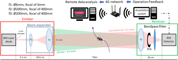
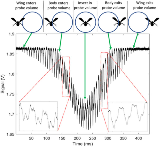
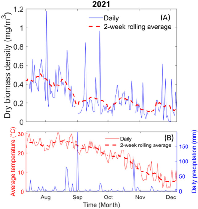
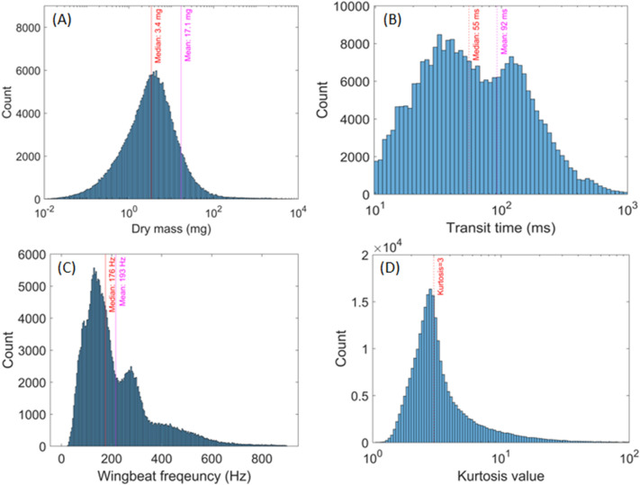
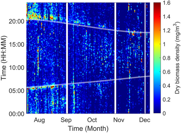
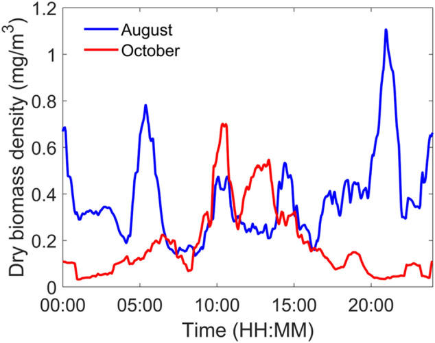
Insects are major actors in Earth's ecosystems and their recent decline in abundance and diversity is alarming. The monitoring of insects is paramount to understand the cause of this decline and guide conservation policies. In this contribution, an infrared laser-based system is used to remotely monitor the biomass density of flying insects in the wild. By measuring the optical extinction caused by insects crossing the 36-m long laser beam, the Entomological Bistatic Optical Sensor System used in this study can evaluate the mass of each specimen. At the field location, between July and December 2021, the instrument made a total of 262,870 observations of insects for which the average dry mass was 17.1 mg and the median 3.4 mg. The daily average mass of flying insects per meter cube of air at the field location has been retrieved throughout the season and ranged between near 0 to 1.2 mg/m³. Thanks to its temporal resolution in the minute range, daily variations of biomass density have been observed as well. These measurements show daily activity patterns changing with the season, as large increases in biomass density were evident around sunset and sunrise during Summer but not during Fall.

Fig. 1

Experimental layout of the Entomological Bistatic Optical Sensor System (eBoss), deployed during the 2021 field campaign. The laser beam is shown in pink and the field of view (FOV) of the receiver in green. The intersection of both defines the probe volume

Fig. 2

Example of an insect signal as the specimen flies through the probe volume of the eBoss. The bottom left and right corners show a magnification of three full wingbeat cycles of the wing contribution. The repeated patterns (136 Hz) are different when the specimen enters and exits the probe volume, which suggests a possible change in the orientation of the specimen

Fig. 3

Noise budget of the experiment. Five different sources of noise have been identified and their respective contribution is expressed in mV and in the percentage of total noise. The range of acquisition was between 0 and 5000 mV, spread over the 2¹⁶ bins of the digitizer. Noise is defined by the standard deviation and the five sources of noise are assumed to be independent and normally distributed

Fig. 4

Top left: satellite view of the area. Top right: aerial view of the field location (40°47′09.8″N 74°03′28.1″W) where both green tents used to protect the equipment from rain can be seen. The optical path of the laser beam is indicated by an orange arrow, starting at the emitter side and pointing toward the receiver side. The weather station, red circle, is located on top of a metal container located directly south of the field. Bottom: picture of the field from the receiver side

Fig. 5

Figure B shows 400 s of raw data, as recorded by the acquisition system, with a sampling frequency of 30,517 Hz. A magnification on one of the identified insect events is displayed as an illustration. Figure A shows the count per bin of intensity and C the spectrogram of the raw data. In the spectrogram, the magnified event stands out and its fundamental frequency as well as its first two harmonics are visible. Figure D shows the optical extinction obtained from figure B, after the application of a digital bandpass filter [10–900 Hz] and averaging. The red line indicates the detection threshold. Any part of the filtered signal that crosses the threshold is identified as a region of interest and the corresponding raw signal is then extracted for further analysis

Fig. 6

Example of two types of signals and their corresponding frequency analysis. Figure A is an example of signal caused by an insect showing clear periodic drop in signal amplitude. Figure C shows its associated Fast Fourier Transform, from which the insect wingbeat frequency can be determined. Figure B is an example of a signal from a non-insect target crossing the probe volume, which does not have any periodic drop in signal amplitude, as can be seen on its Fast Fourier Transform (Figure D)

Fig. 7

Figure A shows a signal due to the crossing of an insect through the probe volume of the eBoss. The red arrow indicates the amplitude of the signal decrease that is due to the body of the insect. $I_0$ is the value of the baseline and $I_{\mathrm{B}}$ is the value taken by the signal when the body of the insect is completely in the center of the probe volume. Figure B shows the same event after conversion in terms of extinction cross section, using Eq. (1)

Fig. 8

Figure A and B display the result of the fit of Eq. (5) for the wet and dry mass, respectively. Error bars represent the standard deviation. Figure C and D display the results of the estimated mass (respectfully wet and dry) using the results of the previous fit, Eqs. (7) and (8), as a function of the actual mass measured with a 0.1 mg precision scale. Each insect group is identified by a unique marker, m for Culicidae, h for Musca domestica, b for Osmia lignaria, w for Vespula maculifrons and bb for Bombus bimaculatus

Fig. 9

In figure A, the solid blue line represents the daily flying insect biomass density per meter cube of air and the red dashed line its 2-week rolling average. The biomass density, expressed in mg/m³, is the dry biomass of the insect. In figure B the solid red line represents the daily average temperature and the dashed red line its 2-week rolling average. The solid blue line represents the daily precipitation

Fig. 10

Figure A displays the distribution of the retrieved mass of insects, using Eq. (8). The median and mean value are displayed in red and magenta, respectively. Figure B shows the distribution of the transit times of insets, i.e., the duration of their transit through the probe volume, which is related to the insect flight velocity. The median and mean value are displayed in red and magenta, respectively. Every event with a transit time lower than 10 ms were systematically removed (hard cut-off at 10 ms). Figure C illustrates the wingbeat frequency distribution of insects. The median and mean value are displayed in red and magenta, respectively. Figure D displays the kurtosis value distribution of every event, which provides information on the shape of the signal. A kurtosis value equal to three, displayed in red, correspond to a Gaussian shape

Fig. 11

Dry biomass density estimation in function of the time-of-day with a 1-min resolution and over the entire measurement campaign of the eBoss. Maximal values of biomass density were artificially capped at 1.6 mg/m³ to improve the color plot contrast. The white lines indicate periods during which the system was offline. The semi-transparent lines indicate the civil sunrise and sunset time at the field location

Fig. 12

Dry biomass density over 24 h. Blue and red line represent the average daily variation of the dry biomass density for the month of August and October, respectively. The presented results are the sixty minutes rolling average of the biomass density, averaged over the entire month

References

1. Ghazoul J. Buzziness as usual ? Questioning the global pollination crisis. Trends Ecol. Evol. 2005 doi: 10.1016/j.tree.2005.04.026. - DOI - PubMed
1. Forister ML, Pelton EM, Black SH. Declines in insect abundance and diversity : we know enough to act now. Conserv. Sci. Pract. 2019 doi: 10.1111/csp2.80. - DOI
1. Wagner DL, Grames EM, Forister ML, Berenbaum MR, Stopak D. Insect decline in the anthropocene: death by a thousand cuts. PNAS. 2021;118:1–10. doi: 10.1073/pnas.2023989118. - DOI - PMC - PubMed
1. Hallmann CA, Sorg M, Jongejans E, Siepel H, Hofland N, Schwan H, et al. More than 75 percent decline over 27 years in total flying insect biomass in protected areas. PLoS ONE. 2017 doi: 10.1371/journal.pone.0185809. - DOI - PMC - PubMed
1. Conrad KF, Warren MS, Fox R, Parsons MS, Woiwod IP. Rapid declines of common, widespread British moths provide evidence of an insect biodiversity crisis. Biol. Conserv. 2006;132:279–291. doi: 10.1016/j.biocon.2006.04.020. - DOI
LinkOut - more resources