Graded optogenetic activation of the auditory pathway for hearing restoration

Abstract

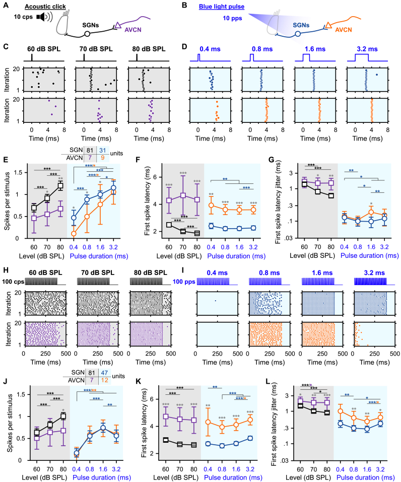
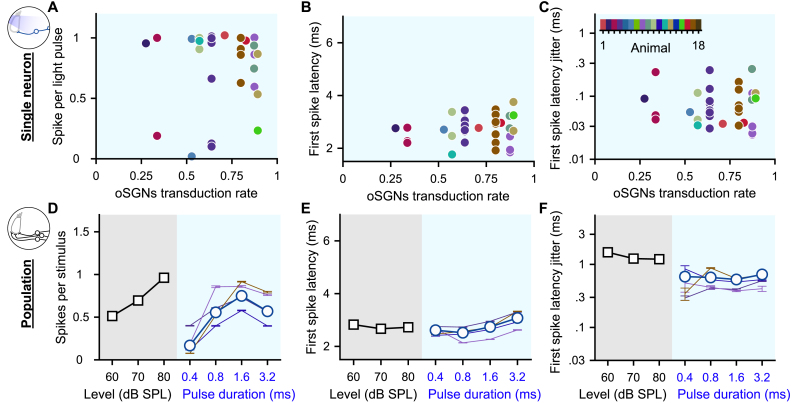
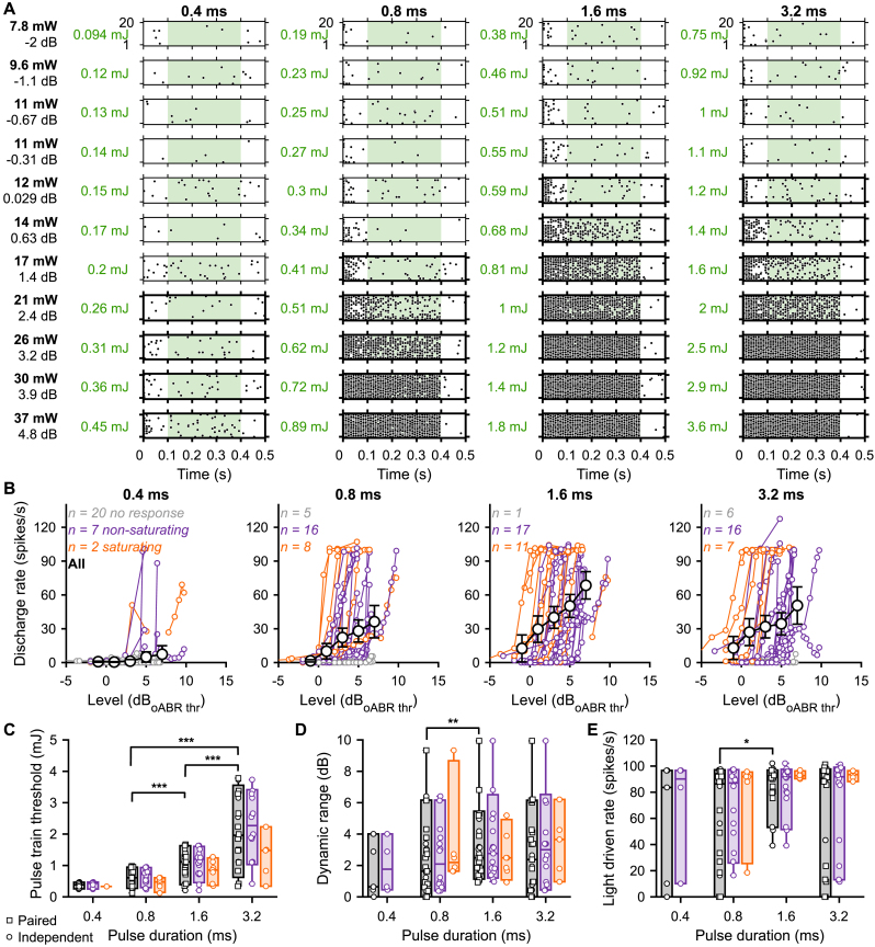
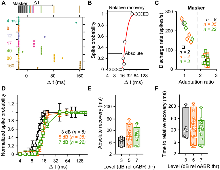
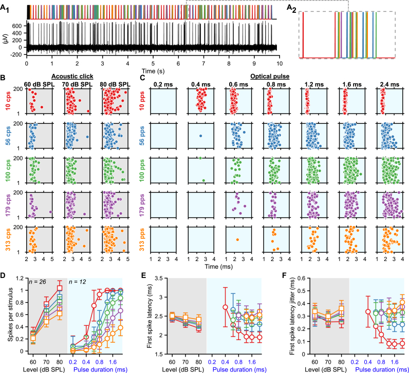
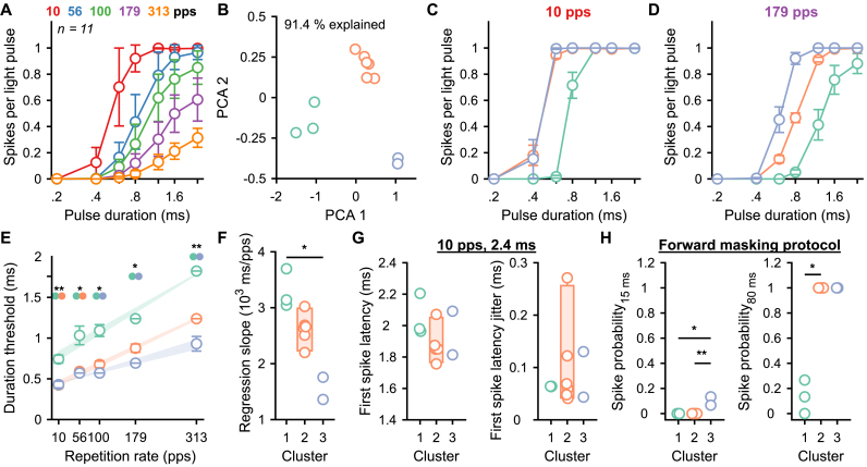
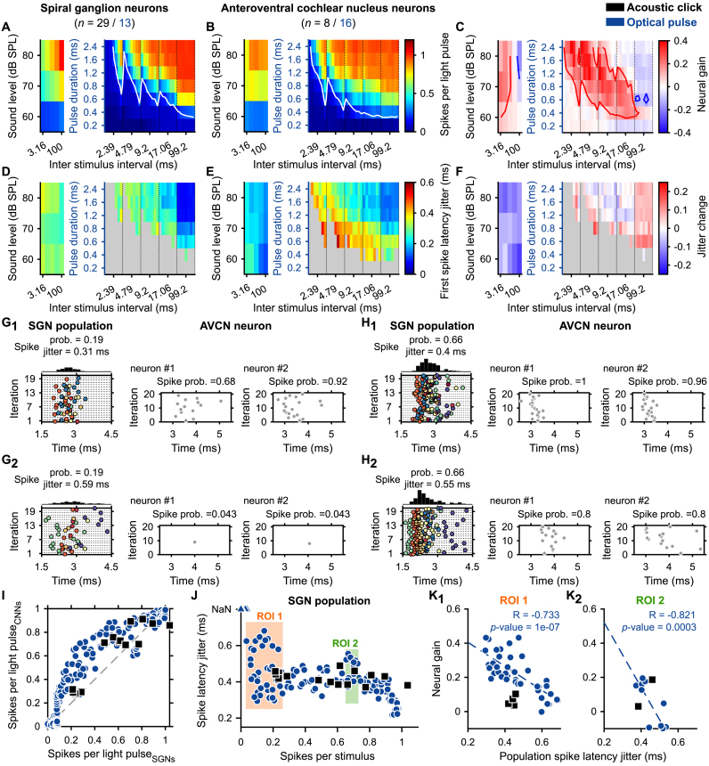
Optogenetic control of neural activity enables innovative approaches to improve functional restoration of diseased sensory and motor systems. For clinical translation to succeed, optogenetic stimulation needs to closely match the coding properties of the targeted neuronal population and employ optimally operating emitters. This requires the customization of channelrhodopsins, emitters and coding strategies. Here, we provide a framework to parametrize optogenetic neural control and apply it to the auditory pathway that requires high temporal fidelity of stimulation. We used a viral gene transfer of ultrafast targeting-optimized Chronos into spiral ganglion neurons (SGNs) of the cochlea of mice. We characterized the light-evoked response by in vivo recordings from individual SGNs and neurons of the anteroventral cochlear nucleus (AVCN) that detect coincident SGN inputs. Our recordings from single SGNs demonstrated that their spike probability can be graded by adjusting the duration of light pulses at constant intensity, which optimally serves efficient laser diode operation. We identified an effective pulse width of 1.6 ms to maximize encoding in SGNs at the maximal light intensity employed here (∼35 mW). Alternatively, SGNs were activated at lower energy thresholds using short light pulses (<1 ms). An upper boundary of optical stimulation rates was identified at 316 Hz, inducing a robust spike rate adaptation that required a few tens of milliseconds to recover. We developed a semi-stochastic stimulation paradigm to rapidly (within minutes) estimate the input/output function from light to SGN firing and approximate the time constant of neuronal integration in the AVCN. By that, our data pave the way to design the sound coding strategies of future optical cochlear implants.

Keywords: Auditory brainstem; Auditory nerve; Chronos; Neural network; Neural stimulation; Neuroprosthetic; Optical cochlear implant; Optogenetics.

Fig. 1

Gradual optogenetic activation of the first neurons of the auditory pathway with light pulses of increasing durations. A-B. Schematic of the in vivo single unit recordings using sharp micropipettes from spiral ganglion neurons (SGNs, black), optogenetically modified SGNs (blue) or neurons of the anteroventral cochlear nucleus (AVCN, acoustic: purple and optogenetic: orange) in response to acoustic click (A) or optogenetic (B) stimulation delivered to the cochlea from an optical fiber (400 ms train stimulation followed by 100 ms silence/dark, 10–20 trials per condition, all data are paired). C-D. Representative raster plots from one SGN (top panel) and one AVCN neuron (bottom panel) in response to single acoustic clicks at various sound pressure levels (C, click trains presented at 10 clicks per second, cps) or single light pulses of different pulse durations (D, ∼35 mW light pulses delivered at 10 pulses per second, pps). Note that acoustic and optogenetic experiments were done from two distinctive cohorts of animals, but SGNs and AVCN neurons were recorded from the same animals respectively. E-G. Quantification of the number of spikes per stimulus (E), first spike latency (F) and first spike latency jitter (G) as a function of the click sound pressure level ("click intensity") for the acoustic modality (grey background) or the light pulse duration for the optogenetic modality (blue background). The color code is similar to panels A–D. The number of units per group is presented in the inset of panel E. Data are represented as mean and confidence interval (95%). The effect of the click intensities and light pulse durations was tested by a Wilcoxon signed rank test on paired samples followed by a Bonferroni correction of the p-values. The difference between SGNs and AVCN neurons was tested by a two-sample t-test or a Wilcoxon rank sum test according to the outcome of Jarque-Bera normality testing (grey symbols; ∗, P ≤ .05; ∗∗, P ≤ .01; ∗∗∗, P ≤ .001). H-L. Same as C-G in response to 100 cps acoustic click or 100 pps light pulse trains. Note that the units presented in H–I are the same as in C-D. (For interpretation of the references to color in this figure legend, the reader is referred to the Web version of this article.)

Fig. 2

Heterogeneous optogenetic activation of the SGNs and artificial population response. A-C. Quantification of the spikes per light pulse (A), first spike latency (B) and first spike latency jitter (C) as a function of the average SGN transduction rate. Measurements were done in response to 100 pps light pulse trains of 1.6 ms (n = 35 SGNs). A color code was used per animal. No correlation was found (correlation coefficient test). D-F. Quantification of the number of spikes per stimulus (D), first spike latency (E) and first spike latency jitter (F) computed across SGNs recorded from a single animal (≥4 SGNs, thin colored line, same color code as in A-C) and all recorded SGNs (grey background, 100 cps acoustic click train: n = 20 SGNs with the best frequency within the 16 kHz octave band; blue background, optogenetics, 100 pps light pulse trais: n = 47 SGNs). (For interpretation of the references to color in this figure legend, the reader is referred to the Web version of this article.)

Fig. 3

The best intensity encoding is achieved using 1.6 ms light pulses. A. Raster plots of a representative SGN evoked by 100 pps light pulse trains (400 ms light, 100 ms dark) at various light intensities and pulse durations. The tested light intensities on the left are expressed in light intensity (or radiant flux in mW), level relative to the oABR threshold (dB_{oABR thr.}, see Methods) and energy (mJ, calculated within the green window, 30 light pulses). Spike trains were computed on the adapted rate (100–400 ms, green window). Tick raster plot boxes highlight response above the threshold which was determined as the light intensities for which d’ ≥ 1 (see Methods). B. Rate level functions of 29 SGNs measured in response to light pulse trains using various light pulse durations. A color code was used to represent non-responding (grey), non-saturating (purple) and saturating (orange) units (see Methods for classification). The average (±95% confidence interval) rate-level function was plotted in black for all pulse durations (intensities values binned between −5 and 8 dB, bin width = 3 dB). Note that the highest light-driven rate was obtained at 1.6 ms. C-E. Quantification of the pulse train threshold (C, 30 light pulses), dynamic range (D) and light-driven rate (E) as a function of the light pulse duration. A color code was used to represent all units (black), non-saturating (purple) and saturating (orange) units Box plots show minimum, 25th percentile, median, 75th percentile, and maximum with individual data points overlaid. Circles represent independent data points and squares paired data points at 0.8, 1.6 and 3.2 ms. The effect of light pulse durations was tested at 0.8, 1.6 and 3.2 ms using a Wilcoxon signed rank test on paired samples followed by a Bonferroni correction. Following assessment for normality using a Jarque-Bera test, the difference between non-saturated and saturated units was tested accordingly by one-way analysis of variance or a Kruskal-Wallis test (∗, P ≤ .05; ∗∗, P ≤ .01; ∗∗∗, P ≤ .001). (For interpretation of the references to color in this figure legend, the reader is referred to the Web version of this article.)

Fig. 4

Recovery from optogenetically induced masking is slow and independent of the stimulation level. SGN firing was fully adapted using a masker (10 light pulses, 316 pps, 1.6 ms duration) and the recovery of firing was assessed at different time intervals (Δ t) ranging between 4 and 200 ms (20 trials, different laser levels ranging between 3 and 6 dB_{rel to oABR threshold}, bin width = 1 dB). A. Representative raster plot of a SGN undergoing the forward masking protocol at 4.67 dB_{rel oABR thr}. A color code is used to represent the different time intervals. B. Recovery curve (i.e. spike probability curve as a function of the time interval) of the unit presented in A. The recovery curve was fitted ($y=\max \left(0,a\times e^{\frac{-\left(k+\Delta t\right)}{b}}\right)$ to define the absolute recovery (i.e. time required to recover any firing, - k) and time to relative recovery (i.e. time required to recover 95% of the spike probability, - k + (3 x b)). C. The discharge rate as a function of the adaptation ratio allowed to cluster SGNs as non-adapted (i.e. adaptation ratio ≤1.8 and discharge rate ≥100 spikes/s) and fully adapted. A color code is used for the different levels (D). D. The average (±95% confidence interval) recovery curve measured from fully adapted SGNs at 3 (black, n = 8), 5 (orange, n = 35), 7 (green, n = 22) dB_{relative to oABR threshold} (bin width = 2 dB). E-F. Quantification of the time to absolute (E) and relative (F) recovery as a function of the light pulse level for the fully adapted SGNs. The same color code is used as in C. Box plots show minimum, 25th percentile, median, 75th percentile, and maximum with individual data points overlaid. No significant difference was observed between the different tested levels (Jarque-Bera test followed by a Kruskal-Wallis test). (For interpretation of the references to color in this figure legend, the reader is referred to the Web version of this article.)

Fig. 5

Input/output function from light to SGN firing can be measured in minutes by a semi-stochastic stimulus. An optical semi-stochastic stimulus (light intensity = 38 mW) was constructed from 20 presentations of random permutation of repetition rates (10, 56, 100, 179, 313 pps and color-coded in the figure) and light pulse durations (0.2, 0.4, 0.6, 0.8, 1.2, 1.6, 2.4 ms). The stochastic stimulus was preceded by a masker (10 light pulses of 0.8 ms) and followed by 200 ms of dark per trial. It was compared to an acoustic stimulus constructed from 20 presentations of acoustic click trains containing random permutations of repetition rates (10, 56, 100, 179, 313 cps) and presented at 60, 70 and 80 dB SPL_PE. Additionally, a forward masking protocol was included in the optogenetic stimulus with time intervals of 15 and 80 ms. A. Single iteration of the optical stochastic stimulus (A₁, top and magnification of the stimulus, A₂) and the response of representative SGNs (A₁, bottom). B–C. Raster plots from representative acoustic (B, grey background) and optically (C, blue background) evoked (o-)SGNs. D-F. Quantification of the number of spikes per stimulus (D), first spike latency (E) and first spike latency jitter (F) as a function of the sound pressure level for the acoustic modality (grey background, n = 26, best frequency within the 16 kHz octave band) and light pulse duration for the optogenetic modality (blue background, n = 13). Data are represented as mean and confidence interval (95%). (For interpretation of the references to color in this figure legend, the reader is referred to the Web version of this article.)

Fig. 6

Heterogeneous responses among SGNs within a single animal. A. Quantification of the number of spikes per light pulse as a function of the repetition rate and light pulse duration from 11 SGNs measured from the same animal. Data are represented as mean and confidence interval (95%). B. The numbers of spikes per light pulse measured at all conditions of repetition rates and light pulse durations were used to perform a principal component analysis (PCA, first 2 components explain 91.4% of the variance) which highlight the presence of 3 SGN clusters (cluster 1, green, n = 3; cluster 2, orange, n = 6; cluster 3, purple, n = 2). C-D. Quantification of the number of spikes per light pulse for the 3 SGN clusters as a function of the light pulse duration at 10 (C) and 179 pps (D). Data are represented as the mean and standard error of the mean. E. Quantification of the light pulse duration threshold as a function of the repetition rate per cluster. The average linear regression (and standard error of the mean) between threshold and repetition rate is represented by the light fill. The threshold difference between clusters was tested using a Kruskal-Wallis test followed by a Tukey's Honestly Significant Difference Procedure (∗, P ≤ .05). F. Quantification of the light pulse threshold dependency on the repetition rate (i.e. the slope of the linear regression between the duration threshold and the repetition rate). Box plots show minimum, 25th percentile, median, 75th percentile, and maximum with individual data points overlaid. The difference between clusters was tested using a Kruskal-Wallis test followed by a Tukey's Honestly Significant Difference Procedure (∗, P ≤ .05; ∗∗, P ≤ .01). G. Quantification of the first spike latency (left) and first spike latency jitter (right) measured in response to the condition: repetition rate = 10 pps and light pulse duration = 2.4 ms per cluster. No difference was measured between clusters (Kruskal-Wallis test). H. Quantification of the spike probability recovery (forward masking protocol as described in Fig. 3) at 15 ms (left) and 80 ms (right) per cluster. (For interpretation of the references to color in this figure legend, the reader is referred to the Web version of this article.)

Fig. 7

The neural gain of the AVCN neurons depended on the level of synchronization between SGNs. The initial 35 conditions of repetition rates and light pulse durations were divided into 245 conditions of inter-stimulus intervals and pulse durations. Note that all conditions were tested randomly for all neurons. A-B, D-E. Quantification of the number of spikes per stimulus (A–B) and first spike latency jitter (D–E) for the different tested conditions for SGNs (A, D, acoustic click, black, n = 29; light pulse, blue, n = 13) and AVCN neurons (B, E, acoustic click, n = 8; light pulse, n = 16). In A-B, the white line delimits the threshold defined as 0.2 spike/stimulus. C,F. Quantification of the neural gain (C) and jitter change (F) between SGNs and AVCN neurons. In C, the red line delimits the area where the neural gain is ≥ 0.1 and the blue line where the neural gain is ≤ 0.1. G. (left) Representative raster plots from 2 illumination conditions eliciting the same spike probability (0.19) within the population of recorded SGNs and two different spike jitters (G₁, 0.31; G₂, 0.59 ms). Individual SGNs are represented by different colors. (right) Raster plots from two AVCN neurons in response to the same illumination conditions. H. Same than G for a spike probability of 0.66 and spike jitters of 0.4 (H₁) and 0.55 ms (H₂). I. Average number of spikes per light pulse of the AVCN neurons as a function of the number of spikes per light pulse of the SGNs. A blue circle (optogenetic) or a black square (acoustic) corresponds to one of the stimulation conditions tested for all neurons. J. First spike latency jitter as a function of the number of spikes per light pulse computed across all SGNs per stimulation condition. Two regions of interest (ROI) were defined as the region where the numbers of spikes per light pulse were in the same range and the variation of the first spike latency jitter was large (ROI 1, 0 ≤ number of spikes per stimulus ≤0.26; ROI 2, 0.65 ≤ number of spikes per stimulus ≤0.73). K. Average neural gain as a function of the first spike latency jitter across SGNs in ROI 1 (K₁) and ROI 2 (K₂). Correlation coefficients (R and its significance) were measured and regressions were displayed as a dashed line if P ≤ .05. (For interpretation of the references to color in this figure legend, the reader is referred to the Web version of this article.)

References

1. Kim C.K., Adhikari A., Deisseroth K. Integration of optogenetics with complementary methodologies in systems neuroscience. Nat Rev Neurosci. 2017;18(4):222–235. - PMC - PubMed
1. Kleinlogel S., Vogl C., Jeschke M., Neef J., Moser T. Emerging approaches for restoration of hearing and vision. Physiol Rev. 2020;100(4):1467–1525. - PubMed
1. Wolf B.J., et al. Is there an unmet medical need for improved hearing restoration? EMBO Mol Med. 2022;14(8) - PMC - PubMed
1. Sahel J.-A., et al. Partial recovery of visual function in a blind patient after optogenetic therapy. Nat Med. 2021;27(7):1223–1229. - PubMed
1. Elkouzi A., Vedam-Mai V., Eisinger R.S., Okun M.S. Emerging therapies in Parkinson disease - repurposed drugs and new approaches. Nat Rev Neurol. 2019;15(4):204–223. - PMC - PubMed
Publication types