Nanoscale structural organization and stoichiometry of the budding yeast kinetochore

Abstract

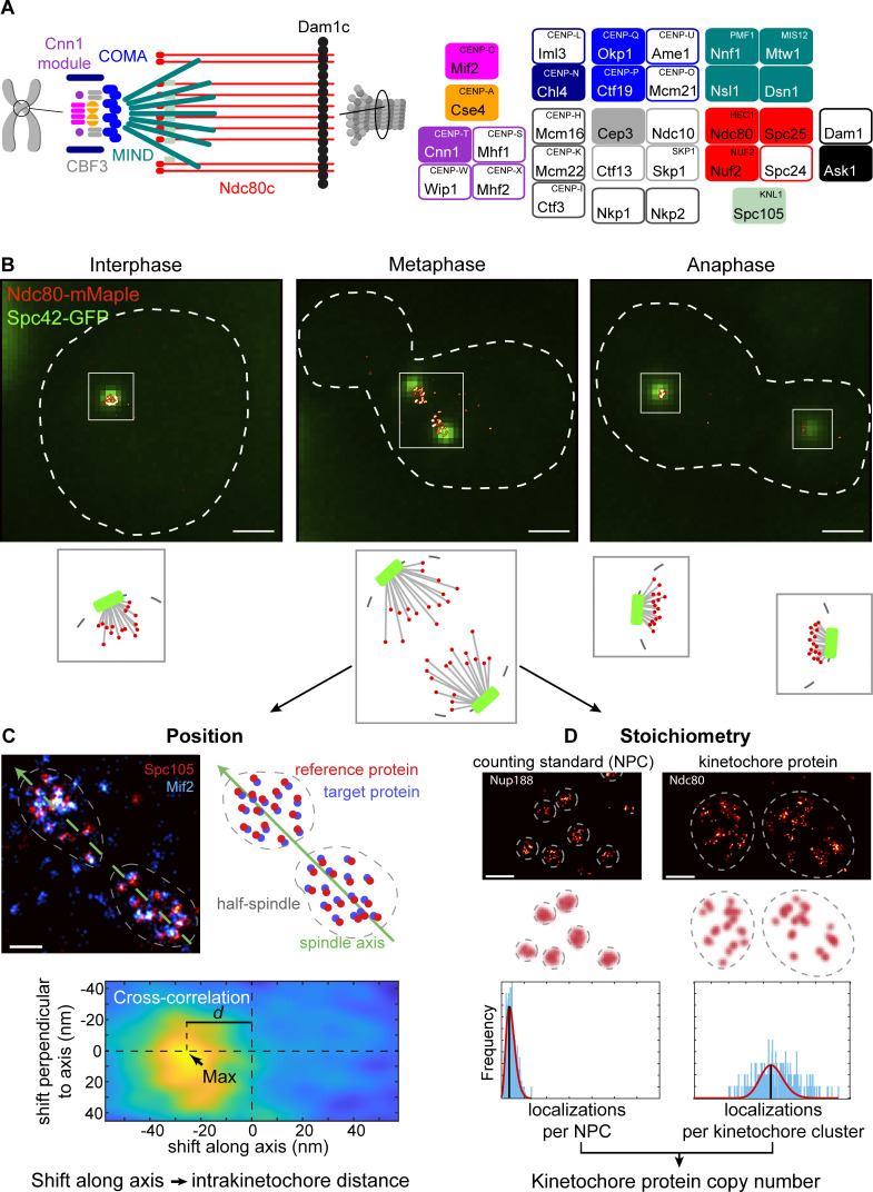
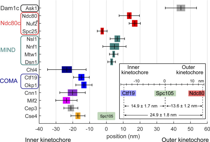
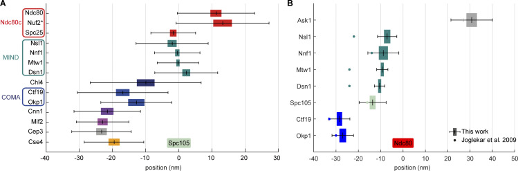
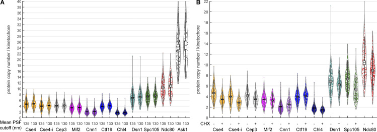
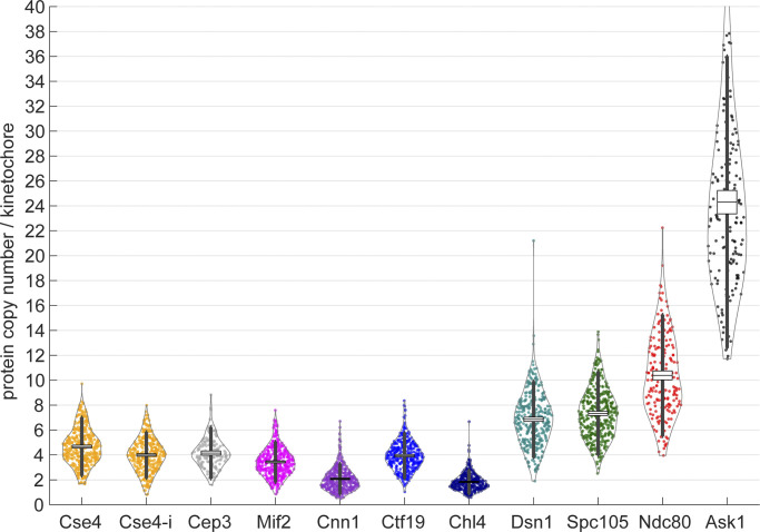
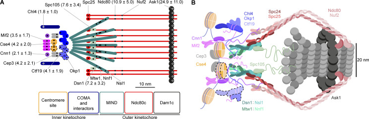
Proper chromosome segregation is crucial for cell division. In eukaryotes, this is achieved by the kinetochore, an evolutionarily conserved multiprotein complex that physically links the DNA to spindle microtubules and takes an active role in monitoring and correcting erroneous spindle-chromosome attachments. Our mechanistic understanding of these functions and how they ensure an error-free outcome of mitosis is still limited, partly because we lack a complete understanding of the kinetochore structure in the cell. In this study, we use single-molecule localization microscopy to visualize individual kinetochore complexes in situ in budding yeast. For major kinetochore proteins, we measured their abundance and position within the metaphase kinetochore. Based on this comprehensive dataset, we propose a quantitative model of the budding yeast kinetochore. While confirming many aspects of previous reports based on bulk imaging, our results present a unifying nanoscale model of the kinetochore in budding yeast.

Figure 1.

Overview of the study. (A) Protein composition of the budding yeast kinetochore. Kinetochore proteins are grouped and color-coded by complexes. Only opaquely colored components were measured in this study. Human counterparts are shown in a superscript. Note that this is not an exhaustive list. (B) Example kinetochore clusters. Overlays of representative super-resolved images of the kinetochore protein Ndc80 (red) and the diffraction-limited images of spindle pole body protein Spc42 (green) at different stages of the cell cycle and corresponding cartoons of the budding yeast spindles. Scale bars: 1 µm. (C) The position of kinetochore proteins along the spindle axis. We always labeled and imaged the reference protein Spc105 (red) together with the target protein (cyan, Mif2 in this example). We manually segmented single kinetochore clusters, defined the spindle axis, and calculated the image cross-correlation. The position of the cross-correlation peak corresponds to the average distance between reference and target proteins in the half spindle. Scale bar: 200 nm. (D) Stoichiometry of the budding yeast kinetochore proteins. We quantified the copy numbers of kinetochore proteins using the NPC component Nup188, which has 16 copies per NPC, as a counting reference standard. In each experiment, we mixed two strains in which either Nup188 or the target kinetochore protein were labeled with the same fluorescence protein tag mMaple. We then imaged both strains simultaneously. We calculated the ratio of mean localization counts per structural unit (either NPC or kinetochore cluster) between the two proteins. From the relative number of localizations and the known stoichiometry of Nup188, we computed the copy number of the target kinetochore protein. Scale bars: 200 nm.

Figure S1.

Workflow of quantifying the distances between kinetochore proteins. (A) Metaphase spindles (white box) with both half spindles close to the focus are manually segmented (dashed contour). The spindle axis for each spindle is manually annotated (green line). A schematic (right panel) is provided for clarity. Scale bars: 1 μm (left), and 500 nm (middle). (B) The overview of the workflow. (C) The distance between the target and reference proteins is quantified using the cross-correlation analysis. This analysis is applied to each kinetochore cluster and yields a correlation map showing the similarity between the two channels at certain lateral and axial shifts of the reference channel. The shift along spindle axis at the maximum is quantified as the distance d. (D) To eliminate the potential offset c caused by the chromatic aberration, the average distances d of both paired kinetochore clusters, having the distances d₁ and d₂ respectively, is then calculated per spindle.

Figure S2.

The basis for defining the values for filtering and quality control. (A–C) Quantifying the width of kinetochore clusters. As shown with the example kinetochore cluster (A), its profile perpendicular to the axis of spindle (B) was fitted with a cylindrical model (red) to quantify the radius. (C) The radius of analyzed kinetochore clusters. The mean radius was quantified as 142.0 ± 23.7 (SD) nm, which corresponds to the width (diameter) of 284 nm. Sample size: 301 kinetochore clusters. (D) The calibration curve (red) relating z positions to PSF size based on bead data (dots). For filtering out out-of-focus localizations, the maximum PSF size of 170 nm is defined, which corresponds to an axial range from −300 to 300 nm. The z ranges bounded by the vertical dashed lines with the same colors [mean PSF size cutoff: 130 nm (orange), 135 nm (blue)] are where kinetochore proteins can be found, given the corresponding mean PSF size cutoffs of kinetochore clusters, taking the quantified width in C into account. Both cutoffs ensure that no analyzed kinetochore protein exceeds the imaging depth determined by the PSF size filtering. (E) The calibration curve relating the z position of a kinetochore cluster to its mean PSF size based on the bead calibration in D. The maximal axial distance between kinetochore clusters in the same pairs $d_z^{max}$ is estimated to be 288 nm, given that the maximal allowed mean PSF size is 135 nm. (F) The relation between the lateral distance d_xy, the axial distance d_z, and the estimated distance between kinetochore clusters in the same pairs d in 3D. Based on the dataset (Ndc80) with the largest sample size, the mean lateral distance between kinetochore clusters in the same pairs ${\overline{d}}_{xy}$ is measured as 777 nm. These correspond to the maximum tilt angle θ^max = 20.3^°, maximum tilt-introduced error of the distance between the kinetochore clusters ϵ^max = 6.3%, and the mean error $\overline{ϵ}=2.1\%$. See Materials and methods for the calculations. Sample size: 50 kinetochore clusters. Scale bars: 200 nm.

Figure 2.

Position of 15 kinetochore proteins along the spindle axis with Spc105 as a reference point. All proteins were tagged at their C-termini. The mean distance is plotted with the SEM (colored box) and SD (whiskers). The inset depicts control measurements showing consistency in pairwise distance measurements ± SEM among three proteins. See Table 1 for values and sample size. *The position of Nuf2 is based on the measured pair Ndc80–Nuf2.

Figure S3.

Intrakinetochore distances measured by different approaches. (A) An independent analysis of intrakinetochore distances based on manually picked single kinetochores. The mean distance is plotted with SEM (as colored box) and SD (whiskers). *The position of Nuf2 was estimated based on Nuf2–Ndc80 distance measurements. (B) Comparison of the available distance measurements to Joglekar et al. (2009). The mean distance is plotted with SEM (as colored box) and SD (whiskers).The corresponding mean values reported by Joglekar et al. (2009) are shown as dots. For comparison, our distance measurements were recalculated using the Ndc80 as the reference point.

Figure S4.

Autocorrelation perpendicular to the spindle axis. Solid curves are average autocorrelation profiles of kinetochore proteins. Dashed lines are autocorrelation profiles of simulated ring distributions with corresponding radii considering the overall distribution of the experimental localization precision.

Figure S5.

Protein copy numbers per kinetochore measured with different filtering or treatments. (A) To investigate the robustness of the molecular counting, different filtering by mean PSF size of kinetochore clusters were applied. Either the kinetochore clusters with PSF size ≤135 or 130 nm were analyzed. The mean protein copy numbers calculated based on both cutoffs are almost identical, showing that the analysis is robust. (B) Cells were treated with or without CHX (250 μg/ml, 60 min) to investigate the effect of protein maturation. Each data point corresponds to one kinetochore cluster. Boxes denote average copy numbers and SEMs, and whiskers denote SDs.

Figure 3.

Protein copy numbers per kinetochore measured with Nup188-mMaple as a counting reference standard. Each data point corresponds to one kinetochore cluster. All proteins were tagged at their C-termini, except Cse4-i that was tagged internally. Boxes denote average copy numbers and SEMs, and whiskers denote SDs. For each protein, two independent experiments were performed and pooled. The pooled copy number and standard deviation were calculated as ${\overline{N}}_k=\sum _j\left(N_{ki}{M}_{ki}\right)/\sum _i{M}_{ki}$ and $\overline{S}=\sqrt{\sum _i{\left(\right(M}_{ki}-1\left)S_i^2\right)/\left(\sum _i{M}_{ki}-I\right),}$ respectively. Here, N_ki, M_ki, and S_i are the copy number, sample size, and SD of the i^th of total I = 2 replicates, respectively. The pooled SEM was given by ${\overline{S}}_m=\overline{S}/\sqrt{\sum _i{M}_{ki}}$ (see Materials and methods for details). Sample size: 389 (Cse4), 347 (Cse4-i), 157 (Cep3), 397 (Mif2), 378 (Cnn1), 357 (Ctf19), 362 (Chl4), 317 (Dsn1), 387 (Spc105), 183 (Ndc80), 156 (Ask1) kinetochore clusters, from two replicates each.

Figure 4.

Structural model of the budding yeast kinetochore. (A) Quantitative schematic model based on the position and protein copy numbers measured with SMLM. The position of the label is shown as a small black dot. Values in the parentheses are the estimates of the number of proteins per kinetochore ± SD. (B) Illustrative structural model that we built by integrating our position and copy number measurements with previous models (Jenni et al., 2017; Fischböck-Halwachs et al., 2019; Hamilton et al., 2019; Ustinov et al., 2020). Dashed lines indicate potentially accessory (non-centromeric) copies (see Results and discussion for details). For simplicity, only two copies of COMA, MIND, and Spc105 and four copies of Ndc80c are shown in B.

References

1. Abbe, E. 1873. Beiträge zur Theorie des Mikroskops und der mikroskopischen Wahrnehmung. Arch. Für Mikrosk. Anat. 9:413–418
1. Ali-Ahmad, A., Bilokapić S., Schäfer I.B., Halić M., and Sekulić N.. 2019. CENP-C unwraps the human CENP-A nucleosome through the H2A C-terminal tail. EMBO Rep. 20:e48913. 10.15252/embr.201948913 - DOI - PMC - PubMed
1. Aravamudhan, P., Felzer-Kim I., Gurunathan K., and Joglekar A.P.. 2014. Assembling the protein architecture of the budding yeast kinetochore-microtubule attachment using FRET. Curr. Biol. 24:1437–1446. 10.1016/j.cub.2014.05.014 - DOI - PMC - PubMed
1. Aravamudhan, P., Goldfarb A.A., and Joglekar A.P.. 2015. The kinetochore encodes a mechanical switch to disrupt spindle assembly checkpoint signalling. Nat. Cell Biol. 17:868–879. 10.1038/ncb3179 - DOI - PMC - PubMed
1. Asbury, C.L. 2017. Anaphase A: Disassembling microtubules move chromosomes toward spindle poles. Biology. 6:15. 10.3390/biology6010015 - DOI - PMC - PubMed
Publication types