Inertialess gyrating engines

Abstract

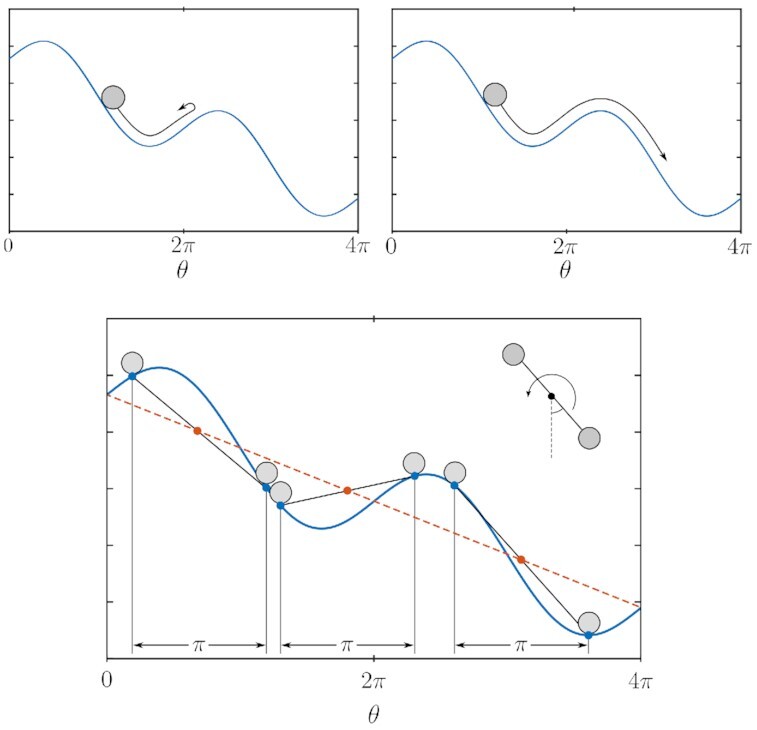
A typical model for a gyrating engine consists of an inertial wheel powered by an energy source that generates an angle-dependent torque. Examples of such engines include a pendulum with an externally applied torque, Stirling engines, and the Brownian gyrating engine. Variations in the torque are averaged out by the inertia of the system to produce limit cycle oscillations. While torque generating mechanisms are also ubiquitous in the biological world, where they typically feed on chemical gradients, inertia is not a property that one naturally associates with such processes. In the present work, seeking ways to dispense of the need for inertial effects, we study an inertia-less concept where the combined effect of coupled torque-producing components averages out variations in the ambient potential and helps overcome dissipative forces to allow sustained operation for vanishingly small inertia. We exemplify this inertia-less concept through analysis of two of the aforementioned engines, the Stirling engine, and the Brownian gyrating engine. An analogous principle may be sought in biomolecular processes as well as in modern-day technological engines, where for the latter, the coupled torque-producing components reduce vibrations that stem from the variability of the generated torque.

Keywords: Brownian gyrator; Stirling engine; averaging; limit cycle oscillation.

Fig.1.

Parts of the Stirling engine and definition of angle θ.

Fig.2.

Top: embodiment of the Brownian gyrator consisting of an RC-circuit. Bottom: Brownian gyrating engine: the rotating wheel couples θ-varying capacitances.

Fig.3.

Potential for the damped pendulum with constant torque. Two cases are displayed. Top-left: inertial effects are not able to overcome the uphills generated by gravity and the only stable solution is the stationary one. Top-right: both inertial effects and constant torque (slope) are enough to sustain continuous motion and the pendulum reaches a stable periodic orbit. Bottom: the average of two potentials displaced by a π phase difference is linear in θ. The graphic representation provides insight into how two θ-equispaced coupled pendula with a constant torque operate stably in a limit cycle: their combined effective potential is a sloped line (red-dashed line in the figure).

Fig.4.

Left: normalized averaged steady state angular velocity vs for one, two, and three coupled engines, with ΔT = 10 K. Note that is normalized by and plotted in a logarithmic scale, where is obtained from [4]. Similarly, the angular velocity is also normalized by . The case with τ = 15 ms is plotted in a dashed line and shows to what extent the assumption of the torque being ω-independent holds. Right: effective potential along two cycles for one, two and three coupled engines.

Fig.5.

Averaged limit cycle angular velocity 〈ω〉 as a function of the temperature difference ΔT for one, two, and three coupled Stirling engines (solid lines). The yellow-dashed line represents the case with τ = 15 ms and three coupled engines, and numerically shows to what extent our assumption of the torque being ω-independent is valid. This agreement is highlighted in the blow-up of the figure. An estimation of the average angular velocity in the limit cycle, based on [4], has been marked by black “×”, showing a good agreement with the numerical results. The (flat) green line corresponds to a stable equilibrium present when the effective torque fails to be sign-definite.

Fig.6.

Left: normalized averaged final angular velocity vs , with ΔT = 10 K for one, two, and three coupled Brownian gyrating engines, respectively. As before, and is as defined in [5]. Right: effective potential along two cycles.

Fig.7.

Average limit cycle angular velocity 〈ω〉 vs ΔT for one, two, and three coupled Brownian gyrating engines. An estimation of the average angular velocity from [5] has been marked by black “×”, matching the numerical results. The (flat) green line corresponds to a stable equilibrium present when the effective torque fails to be sign-definite.

References

1. Toyabe S, Izumida Y. 2020. Experimental characterization of autonomous heat engine based on minimal dynamical-system model. Phys Rev Res. 2: 033146.
1. Miangolarra OM, Taghvaei A, Chen Y, Georgiou TT., 2022. Thermodynamic engine powered by anisotropic fluctuations. Phys Rev Res. 4: 023218.
1. Meister M, Lowe G, Berg HC., 1987. The proton flux through the bacterial flagellar motor. Cell. 49(5): 643–650. - PubMed
1. Noji H, Yasuda R, Yoshida M, Kinosita K., 1997. Direct observation of the rotation of F1-ATPase. Nature. 386(6622): 299–302. - PubMed
1. Kay ER, Leigh DA, Zerbetto F., 2007. Synthetic molecular motors and mechanical machines. Angew Chem Int Edn. 46(1–2): 72–191. - PubMed
LinkOut - more resources