Memorizing without overfitting: Bias, variance, and interpolation in overparameterized models

Abstract

The bias-variance trade-off is a central concept in supervised learning. In classical statistics, increasing the complexity of a model (e.g., number of parameters) reduces bias but also increases variance. Until recently, it was commonly believed that optimal performance is achieved at intermediate model complexities which strike a balance between bias and variance. Modern Deep Learning methods flout this dogma, achieving state-of-the-art performance using "over-parameterized models" where the number of fit parameters is large enough to perfectly fit the training data. As a result, understanding bias and variance in over-parameterized models has emerged as a fundamental problem in machine learning. Here, we use methods from statistical physics to derive analytic expressions for bias and variance in two minimal models of over-parameterization (linear regression and two-layer neural networks with nonlinear data distributions), allowing us to disentangle properties stemming from the model architecture and random sampling of data. In both models, increasing the number of fit parameters leads to a phase transition where the training error goes to zero and the test error diverges as a result of the variance (while the bias remains finite). Beyond this threshold, the test error of the two-layer neural network decreases due to a monotonic decrease in both the bias and variance in contrast with the classical bias-variance trade-off. We also show that in contrast with classical intuition, over-parameterized models can overfit even in the absence of noise and exhibit bias even if the student and teacher models match. We synthesize these results to construct a holistic understanding of generalization error and the bias-variance trade-off in over-parameterized models and relate our results to random matrix theory.

FIG. 1.. Double-descent phenomenon.

(a)-(b) Examples of the average training error (blue squares) and test error (black circles) for two different models calculated via numerical simulations. In both models, the test error diverges when the training error reaches zero at the interpolation threshold, located where the number of parameters N_p matches the number of points in the training data set M (indicated by a black dashed vertical line). (a) In linear regression without basis functions, the number of features in the data N_f matches the number of fit parameters N_p. (b) The random nonlinear features model (two-layer neural network where the parameters of the middle layer are random but fixed) decouples the number of features N_f and the number of fit parameters N_p by incorporating an additional “hidden layer” and transforms the data using a nonlinear activation function (e.g., ReLU), resulting in the canonical double-descent behavior. (c) Schematic of the model architecture for the random nonlinear features model. Numerical results are shown for a linear teacher model $y(\overrightarrow{\mathbf{\text{x}}})=\overrightarrow{\mathbf{\text{x}}}\cdot \overrightarrow{\mathit{\beta }}+\epsilon$, a signal-to-noise ratio of ${\sigma }_{\beta }^2{\sigma }_X^2/{\sigma }_{\epsilon }^2=10$, and a small regularization parameter of λ = 10⁻⁶. The y-axes have been scaled by the variance of the training set labels ${\sigma }_y^2={\sigma }_{\beta }^2{\sigma }_X^2+{\sigma }_{\epsilon }^2$. Each point is averaged over at least 1000 independent simulations trained on M = 512 data points with small error bars indicating the error on the mean. In (b), there are less features than data points N_f = M/4. See Sec. II for precise definitions and Sec. S4 of Supplemental Material [5] for additional simulation details.

FIG. 2.. Linear Regression (No Basis Functions).

Analytic solutions for the ensemble-averaged (a) training error (blue squares) and test error (black circles), and (b) bias-variance decomposition of test error with contributions from the squared bias (blue squares), variance (red squares), and test set label noise (green triangles), plotted as a function of α_f = N_f/M (or equivalently, α_p = N_p/M). Analytic solutions are indicated as dashed lines with numerical results shown as points with small error bars indicating the error on the mean. In each panel, a black dashed vertical line marks the interpolation threshold α_f = 1. (c) Analytic solution for the minimum eigenvalue ${\sigma }_{\text{min}}^2$ of the Hessian matrix Z^TZ. Examples of the eigenvalue distributions are shown (i) in the under-parameterized regime with α_f = 1/8, (ii) at the interpolation threshold, α_f = 1, and (iii) in the over-parameterized regime with α_f = 8. Analytic solutions for the distributions are depicted as black dashed curves with numerical results shown as blue histograms. See Sec. S4 of Supplemental Material [5] for additional simulation details.

FIG. 3.. Random Nonlinear Features Model (Two-layer Neural Network).

Analytic solutions for the ensemble-averaged (a) training error (blue squares) and test error (black circles), and (b) bias-variance decomposition of test error with contributions from the squared bias (blue squares), variance (red squares), and test set label noise (green triangles), plotted as a function of α_p = N_p/M for fixed α_f = N_f/M = 1/4. Analytic solutions are indicated as dashed lines with numerical results shown as points. Analytic solutions as a function of both α_p and α_f are also shown for the the ensemble-averaged (c) training error, (d) test error, (e) squared bias, and (f) variance. In all panels, a black dashed line marks the boundary between the under- and over-parameterized regimes at α_p = 1. (g) Analytic solution for the minimum eigenvalue ${\sigma }_{\text{min}}^2$ of the Hessian matrix Z^TZ. Examples of the eigenvalue distributions are shown (i) in the under-parameterized regime with α_p = 1/8, (ii) at the interpolation threshold, α_p = 1, and (iii) in the over-parameterized regime with α_p = 8, all for α_p = 1/4. Analytic solutions for the distributions are shown as blacked dashed curves with numerical results shown as blue histograms. See Sec. S4 of Supplemental Material [5] for additional simulation details.

FIG. 4.. Poorly sampled directions in space of features lead to overfitting.

Demonstrations of this phenomenon are shown for (a) linear regression and (b) the random nonlinear features model. Columns (i), (ii), and (iii) correspond to models which are under-parameterized, exactly at the interpolation threshold, or over-parameterized, respectively. In each example, the relationship between the labels and the projection of their associated input or hidden features onto the minimum principal component ĥ_min of Z^TZ is depicted for a set of training data (orange squares) and a test set (blue circles). Orange lines indicate the relationship learned by a model from the training set, while the expected relationship for an average test set is shown as a blue line. In the left-most column, the spread (standard deviation) of an average training set along the x-axis, ${\sigma }_{\text{train}}^2={\sigma }_{\text{min}}^2/M$, is plotted relative to the spread that would be expected for an average test set, ${\sigma }_{\text{test}}^2$, for simulated data as a function of α_p. Smaller values are associated with lower prediction accuracy on out-of-sample data, coinciding with small eigenvalues in Z^TZ. All results are shown for a linear teacher model. See Supplemental Material [5] for analytic derivations of learned and expected relationships and spreads along minimum principal components (Sec. S3), along with additional details of numerical simulations (Sec. S4).

FIG. 5.. Biased models can interpret signal as noise.

(a) The total bias (black circles) with contributions from the linear label components (blue squares) and nonlinear label components (red diamonds), and the (b) the total variance (black circles) with contributions from the linear label components (blue squares), nonlinear label components (red diamonds), and the label noise (green triangles) are shown for linear regression with a nonlinear teacher model f(h) = tanh(h) [see Eq. (2)]. Analytic solutions are indicated as dashed lines with numerical results shown as points. Contributions from the linear label components, nonlinear label components, and label noise are found by identifying terms in the analytic solutions proportional to ${\sigma }_{\beta }^2{\sigma }_X^2$, ${\sigma }_{\delta y^{*}}^2$, and ${\sigma }_{\epsilon }^2$, respectively. Each source of bias acts as effective noise, giving rise to a corresponding source of variance. The effects of this phenomenon on the relationships learned by a linear regression model are depicted at the interpolation threshold for an unbiased model with linear data, f(h) = h, (c) with noise and (d) without noise, and for a biased model with nonlinear data, f(h) = tanh(h), (e) with noise and (f) without noise. In each example, the relationship between the labels and the projection of their associated input features onto the minimum principal component ${\widehat{\mathbf{\text{h}}}}_{\text{min}}$ of X^TX is depicted for a set of training data (orange squares) and a test set (blue circles). Orange lines indicate the relationship learned by a model from the training set, while the expected relationship for an average test set is shown as a blue line. See Supplemental Material [5] for analytic derivations of learned and expected relationships (Sec. S3), along with additional details of numerical simulations (Sec. S4).

FIG. 6.. Susceptibilities for Random Nonlinear Features Model.

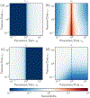
Analytic solutions for three key susceptibilities as a function of α_p = N_p/M and α_f = N_f/M. (a)–(b) The susceptibility ν measures the sensitivity of the fit parameters with respect to small perturbations in the gradient. In the small λ limit, we make the approximation ν ≈ λ⁻¹ν₋₁ + ν₀. (a) The coefficient ν₋₁ characterizes over-parameterization, equal to the the fraction of fit parameters in excess of that needed to achieve zero training error. (b) The coefficient ν₀ characterizes overfitting, diverging at the interpolation threshold when Z^TZ has a small eigenvalue. (c) The susceptibility χ measures the sensitivity of the residual label errors of the training set to small perturbations in the label noise. As a result, χ characterizes interpolation, equal to the fraction of data points that would need to be removed from the training set to achieve zero training error. (d) The susceptibility κ measures the sensitivity of the residual parameter errors to small perturbations in the ground truth parameters. We observe that κ decreases as a model becomes less biased, indicating that the model is better able to express the relationships underlying the data. In each panel, a black dashed line marks the boundary between the under- and over-parameterized regimes at α_p = 1.

References

1. Lecun Yann, Bengio Yoshua, and Hinton Geoffrey, “Deep learning,” Nature 521, 436–444 (2015). - PubMed
1. Canziani Alfredo, Paszke Adam, and Culurciello Eugenio, “An Analysis of Deep Neural Network Models for Practical Applications,” (2017), arXiv:1605.07678.
1. Zhang Chiyuan, Bengio Samy, Hardt Moritz, Recht Benjamin, and Vinyals Oriol, “Understanding Deep Learning Requires Re-thinking Generalization,” International Conference on Learning Representations (ICLR) (2017).
1. Mehta Pankaj, Bukov Marin, Wang Ching Hao, Day Alexandre G.R., Richardson Clint, Fisher Charles K., and Schwab David J., “A high-bias, low-variance introduction to Machine Learning for physicists,” Physics Reports 810, 1–124 (2019). - PMC - PubMed
1. “See supplemental material at [url] for complete analytic derivations and additional numerical results.”.
LinkOut - more resources