Electromagnetic Forces and Torques: From Dielectrophoresis to Optical Tweezers
- PMID: 36719985
- PMCID: PMC9951227
- DOI: 10.1021/acs.chemrev.2c00576
Electromagnetic Forces and Torques: From Dielectrophoresis to Optical Tweezers
Abstract
Electromagnetic forces and torques enable many key technologies, including optical tweezers or dielectrophoresis. Interestingly, both techniques rely on the same physical process: the interaction of an oscillating electric field with a particle of matter. This work provides a unified framework to understand this interaction both when considering fields oscillating at low frequencies─dielectrophoresis─and high frequencies─optical tweezers. We draw useful parallels between these two techniques, discuss the different and often unstated assumptions they are based upon, and illustrate key applications in the fields of physical and analytical chemistry, biosensing, and colloidal science.
Conflict of interest statement
The authors declare no competing financial interest.
Figures


 and
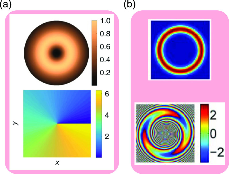
and  > 0. (b) Negative intensity and phase gradient
forces for
> 0. (b) Negative intensity and phase gradient
forces for  and
and  < 0.
< 0.


 is a vector coming out of the page toward
the reader.
is a vector coming out of the page toward
the reader.


References
Publication types
LinkOut - more resources
Full Text Sources