Spatially resolved transcriptomic profiling of degraded and challenging fresh frozen samples

Abstract

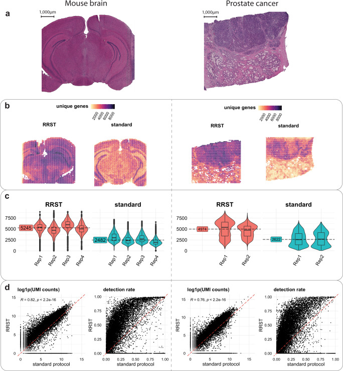
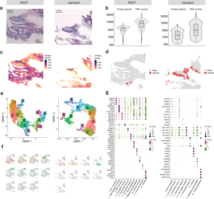
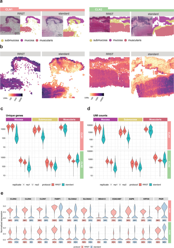
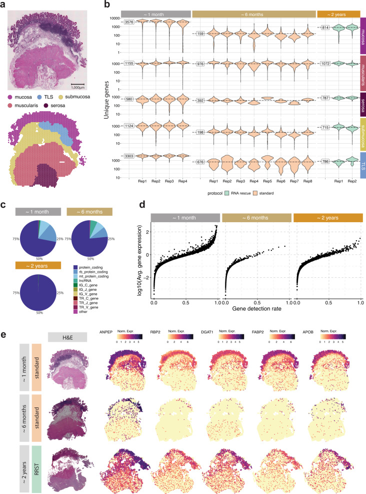
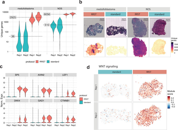
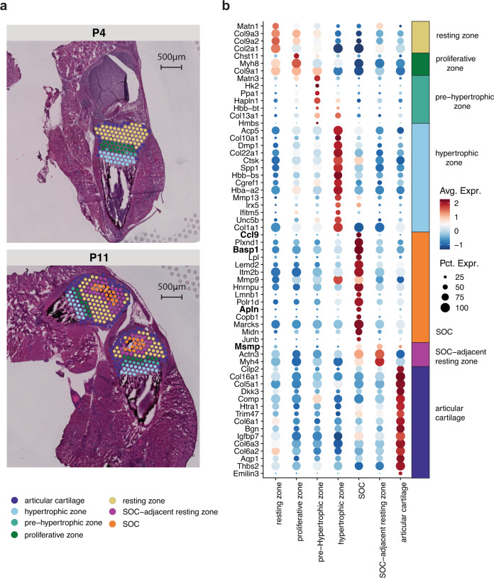
Spatially resolved transcriptomics has enabled precise genome-wide mRNA expression profiling within tissue sections. The performance of methods targeting the polyA tails of mRNA relies on the availability of specimens with high RNA quality. Moreover, the high cost of currently available spatial resolved transcriptomics assays requires a careful sample screening process to increase the chance of obtaining high-quality data. Indeed, the upfront analysis of RNA quality can show considerable variability due to sample handling, storage, and/or intrinsic factors. We present RNA-Rescue Spatial Transcriptomics (RRST), a workflow designed to improve mRNA recovery from fresh frozen specimens with moderate to low RNA quality. First, we provide a benchmark of RRST against the standard Visium spatial gene expression protocol on high RNA quality samples represented by mouse brain and prostate cancer samples. Then, we test the RRST protocol on tissue sections collected from five challenging tissue types, including human lung, colon, small intestine, pediatric brain tumor, and mouse bone/cartilage. In total, we analyze 52 tissue sections and demonstrate that RRST is a versatile, powerful, and reproducible protocol for fresh frozen specimens of different qualities and origins.

Fig. 1. Comparison of RRST and Visium on mouse brain and prostate tumor samples.

a H&E images of a representative tissue section from mouse brain (left) and prostate cancer (right). The entire dataset consisted of 8 consecutive mouse brain tissue sections and 4 consecutive prostate cancer tissue sections. Half of the tissue sections were processed with RRST and the remaining half with standard Visium protocol. b Spatial distribution of unique genes in two representative tissue sections for each tissue type, one processed with the RRST protocol and one processed with the standard Visium protocol. c Distributions of unique genes per spot visualized as violin/box plots colored by experimental protocol for mouse brain and prostate cancer data. Box plots are presented as median values where the lower and upper bounds are the 25th and 75th percentiles. The upper and lower limits of the boxplots are defined by the closest value no further than 1.5*IQR (inter-quartile range) from the closest bound. Values outside of the upper and lower limits are highlighted as outliers. The median number of unique genes is highlighted for each group (sample type and protocol) next to the violin plots. d gene-gene scatter plots between RRST data (y-axis) and standard Visium data (x-axis) of log1p-transformed UMI counts and detection rates using the data shown in (b). The UMI counts and detection rates were calculated across the pooled technical replicates within each experimental protocol. The red dashed line highlights a 1-to-1 relationship. For the log1p-transformed UMI counts scatter plot, only genes targeted by the probe panel were included. The detection rate for a gene is defined as the proportion of spots with detected UMI counts. The statistical test is based on the Pearson product moment correlation coefficient and p-values were estimated using a two-sided alternative hypothesis.

Fig. 2. RRST and standard Visium applied to human adult lung tissue.

Each subplot shows the RRST data on the left side and the standard Visium data on the right side. a H&E images of two representative tissue sections collected from the same tissue block. b Violin/box plots showing the distribution of unique genes and UMI counts for RRST (n = 1) and standard Visium (n = 2) data generated from consecutive tissue sections from the same lung tissue specimen. The y-axis is shown in log10 scale. Box plots are presented as median values where the lower and upper bounds are the 25th and 75th percentiles. The upper and lower limits of the boxplots are defined by the closest value no further than 1.5*IQR (inter-quartile range) from the closest bound. Values outside of the upper and lower limits are highlighted as outliers. c Unique genes per spot mapped on tissue coordinates. d Spatial visualization showing what spots were discarded due to low quality (less than 300 unique genes detected). e UMAP embedding of adult lung data colored by clusters detected by unsupervised graph-based clustering (louvain). f Split view of clusters (same as in e) mapped on tissue coordinates. g Dot plots of the top marker genes for each cluster. Each cluster was annotated based on its spatial localization in the tissue and expression of canonical marker genes.

Fig. 3. Comparison of data quality in RRST and standard Visium datasets generated from adult human colon tissues.

a Representative H&E images and annotated regions for two patient samples processed by either RRST (n = 4) or standard Visium (n = 2) protocol. The spots in each tissue section were labeled into three categories: mucosa, submucosa, and muscularis. b Distribution of UMI counts in the tissue sections shown in (a). The color scale represents log10-transformed counts. c Distribution of unique genes per spot in the three annotated regions (mucosa, submucosa, and muscularis) visualized as violin plots, for all tissue sections. The y-axis shows log10-transformed counts. d Distribution of UMI counts per spot in the three annotated regions (mucosa, submucosa, and muscularis) visualized as violin plots. The y-axis shows log10-transformed counts. e Expression of 11 epithelial markers in the mucosa for the two adult colon samples visualized as violin plots. A comparison between the two protocols is shown for each gene and the corresponding detection rate is highlighted below each violin plot. The detection rate is defined as the percentage of spots (in the mucosa) where the gene is detected.

Fig. 4. Comparison between RRST and standard Visium on an adult human small intestine sample over time.

a Representative H&E image (top) and spots colored by five major tissue regions (bottom): mucosa, TLS, submucosa, muscularis, and serosa. TLS, Tertiary Lymphoid Tissue. The full small intestine dataset consisted of 14 tissue sections collected from the same specimen at different time points. Only sections collected at the last point were processed with RRST, while the other sections were processed with standard Visium protocol. b Overview of data quality in the five annotated tissue regions over time, visualized by violin plots of the number of unique genes per spot. The time points represent the approximate storage time after sample collection: ~1 month, ~6 months, and ~2 years. Replicates obtained for each time point are shown on the x-axis. The fill color of the violin plots indicates the applied protocol. For each time point, labels on the left side of the violin plots represent the average over all replicates. c RNA biotype content for the three datasets visualized as a pie chart. Proportions represent the UMI counts detected for each biotype. The targeted RRST data include protein coding, immunoglobulin, and T-cell receptor transcripts. d Mean-detection rate relationship in the mucosa for data collected at the three different time points. The y-axis shows log10-transformed average number of UMIs for each gene, and the x-axis shows the detection rate for each gene. The detection rate is defined as the fraction of spots where the gene is detected. e Spatial visualization of five enterocyte markers. Each row represents one selected tissue section from each time point with their corresponding H&E image in the leftmost column. Spot colors represent normalized gene expression.

Fig. 5. Comparison between standard Visium and RRST protocols in eight pediatric brain tumor tissue sections.

a Violin plots showing the number of unique genes per spot in all eight tissue sections (medulloblastoma n = 4, NOS n = 4). The fill color represents the protocol used to generate the data. The average number of unique genes for each sample and protocol are highlighted by dashed lines. The y-axis shows log10-transformed values. b H&E images (top row) and the number of unique genes per spot (bottom row) shown for four representative tissue sections. c Violin plots showing the normalized expression of 6 marker genes related to WNT-signaling across the four medulloblastoma tissue sections. The fill color represents the protocol used to generate the data. Rep1, replicate 1; Rep2, replicate 2. Norm. Expr., normalized gene expression. d Spatial visualization of WNT-signaling module scores in the WNT medulloblastoma samples.

Fig. 6. Comparison of standard Visium with RRST on mouse cartilage tissue.

a Average numbers of unique genes are highlighted by dashed lines for each protocol next to the violin plots. The y-axis represents log10-scaled counts. 1 tissue section was processed with the standard Visium protocol for P4 and P11, and 2 tissue sections for each timepoint (P4, P11) with the RRST protocol. b Following NNMF, Factors 12 and 2 associated with resting and proliferating chondrocytes. c Factors 1 and 11 associated with hypertrophic chondrocytes and primary spongiosa. d Factor 6 associated with the cruciate ligament. e Factor 7 associated with Perichondrium and periosteum. Spot colors represent the factor activity, i.e., the contribution of each spot to the factor. The spot opacity has been scaled by the factor activity scores, making spots with lower scores more transparent.

Fig. 7. Investigating the potential secreted markers within mouse cartilage at 2 postnatal time points.

a Comparing the manually assigned sub-clusters between postnatal day 4 and day 11. b Differentially upregulated genes listed from highest to lowest fold change within each annotated region (avg_log2FC > 0.6 and a maximum of 15 genes per region).

References

1. Larsson L, Frisén J, Lundeberg J. Spatially resolved transcriptomics adds a new dimension to genomics. Nat. Methods. 2021;18:15–18. - PubMed
1. Rao A, Barkley D, França GS, Yanai I. Exploring tissue architecture using spatial transcriptomics. Nature. 2021;596:211–220. - PMC - PubMed
1. Moses L, Pachter L. Museum of spatial transcriptomics. Nat. Methods. 2022;19:534–546. - PubMed
1. Maniatis S, et al. Spatiotemporal dynamics of molecular pathology in amyotrophic lateral sclerosis. Science. 2019;364:89–93. - PubMed
1. Asp M, et al. A spatiotemporal organ-wide gene expression and cell atlas of the developing human heart. Cell. 2019;179:1647–1660.e19. - PubMed
Publication types