Salp blooms drive strong increases in passive carbon export in the Southern Ocean

Abstract

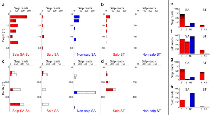
The Southern Ocean contributes substantially to the global biological carbon pump (BCP). Salps in the Southern Ocean, in particular Salpa thompsoni, are important grazers that produce large, fast-sinking fecal pellets. Here, we quantify the salp bloom impacts on microbial dynamics and the BCP, by contrasting locations differing in salp bloom presence/absence. Salp blooms coincide with phytoplankton dominated by diatoms or prymnesiophytes, depending on water mass characteristics. Their grazing is comparable to microzooplankton during their early bloom, resulting in a decrease of ~1/3 of primary production, and negative phytoplankton rates of change are associated with all salp locations. Particle export in salp waters is always higher, ranging 2- to 8- fold (average 5-fold), compared to non-salp locations, exporting up to 46% of primary production out of the euphotic zone. BCP efficiency increases from 5 to 28% in salp areas, which is among the highest recorded in the global ocean.

Fig. 1. Study area.

Lagrangian sampling (tracks shown as red lines/dots). Water mass types: Subantarctic Southland Current (SA-Sc), Subantarctic (SA), and Subtropical (ST). The location of the bathymetric feature is labeled “Chatham Rise” and extends to the east of the Chatham Islands, and the island of New Zealand is to the west of the study location. Colors indicate sea surface temperature (see color bar).

Fig. 2. Phytoplankton community metrics.

a Depth-resolved size-composition (0.2–2 µm, 2–20 µm, >20 µm) of chlorophyll a (see legend for colors) for each experimental cycle. Note different scales on x axis. Mixed layer is denoted by the straight line (shallower depth), and euphotic zone (0.1% PAR) by the dashed line (deeper depth). b Autotrophic integrated community composition: size-fractionated chlorophyll a (color-coded as in (a), pigment-based composition, and DNA-based composition, with colors corresponding to legend specifications. c PSII maximum quantum yield: phytoplankton physiology indicated by the Photosystem 2 (PSII) maximum quantum yield (Fv/Fm) and reoxidation kinetics (Q_a^—lifetime), and Phytoplankton growth and grazing: net primary productivity (NPP) and phytoplankton biomass accumulation (NPP—μzoo grazing). Errors are standard deviation. Symbols and colors are indicated in the legend: red markers indicate salp bloom locations, blue markers indicate non-salp locations, circles are for Subantarctic Southland Current (SA-Sc), squares are for Subantarctic (SA) waters, and diamonds are for Subtropical (ST) waters.

Fig. 3. Simplified schematic of the life cycle of salps.

The oozooid refers to the asexual (or solitary) stage. The oozooid begins to produce chains of blastozooid clones (also known as the sexual or aggregate phase) typically in response to enhanced phytoplankton biomass, triggering the onset of a bloom. Once blastozooids reach maturity they each harbors one oozooid embryo, which is birthed live. After releasing the embryo, the female blastozooids mature their male testis (not shown here), and the cycle is completed with the maturation of the young oozooid. The length of the entirety of the cycle for S. thompsoni in Antarctic waters (−1–2 °C) has been estimated to range between 2 and 9 months depending on the study, although the generation time of the blastozooids is much shorter compared to oozooids. Growth rates of blastozooids during SalpPOOP suggest a shorter life-cycle duration in the warmer waters (~10 °C) of the Chatham Rise, ranging between 12 and 42 days (average 23). The blastozooids emerge as <1 mm sized animals and continue to grow to ~50 mm when mature females.

Fig. 4. Size-specific salp abundance and fecal pellet production rates.

a Abundance (day/night averaged) of salps in the upper 200 m, and b fecal pellet production (Fprod_Gpig) rates by size class for the four salp locations. Green bars correspond to oozooids and brown bars correspond to blastozooids. Error bars for all panels are SE.

Fig. 5. Patterns in carbon export flux.

Mean ± std of a export fluxes of particulate organic carbon (POC), b carbon flux due to recognizable salp fecal pellets (FP), c relative contribution of intact salp FP to POC flux. Colors and symbols for experimental cycles are denoted in the legend in (a). d Ratio of POC flux between Salp and non-salp locations, with three comparisons for SA waters, and one for ST waters. Doted line indicates a ratio of 1. e E_Z ratio, the ratio of POC flux: net primary production (NPP), as a function of T₁₀₀ (POC flux at E_Z + 100 m/POC flux). Numbers indicate locations compared in ref. : 1—North Atlantic Bloom Experiment (NABE) (spring, temperate North Atlantic), 2—Kiwi 7, 3—Kiwi 8 (Polar Front, Pacific sector, Southern Ocean), 4—K2 - D1 (subarctic NW Pacific), 5—K2 - D2 (subarctic, NW Pacific), 6—ALOHA (subtropical, central North Pacific), 7—EqPac (tropical, central Pacific), 8—OSP – Aug (summer, NE Pacific), 9—OSP – May (spring, NE Pacific). Circles are proportional to magnitude of NPP (see legend insert). Results from this study are in color: blue indicates non-salp locations, red indicates salp cycles during the SalpPOOP experiment.

Fig. 6. ²³⁴Th flux out of the upper ocean.

x axis indicates Th-234 flux estimates measured in PIT, while y axis indicates Th-234 flux estimates using the ²³⁸U:²³⁴Th disequilibrium method, using water profiles of Th-234 and salinity-derived U-238 estimates, with integration depths matching the depth of the Particle Interceptor Traps (PIT). Filled markers indicate values estimated using steady-state assumptions, open markers (Salp Subantarctic, Salp SA) indicate non-steady state assumptions (box above break). Note scale change for the non-steady state. Error bars are 1 std propagated from all uncertainty terms.

Fig. 7. Non-metric multidimensional scaling (NMDS) of microbial communities during SalpPOOP.

a Protistan communities sampled in Particle Interceptor Traps (PIT), b Protistan communities in the euphotic zone of the water column (WC) sampled from the conductivity–temperature-depth CTD rosette, and c Bacteria/Archaea communities in the euphotic zone of the water column (also sampled from the CTD). Water mass explained most of the variance among communities in the different locations—PIT protists: 7% variance, WC protists: 19%, WC prokaryotes: 20% (PERMANOVA, all P values «0.001). Salp/non-salp followed for protists (PIT: 4% variance, WC: 9% variance), and was also significant for prokaryotes (7.6% variability). Depth of collection explained similar levels of variability in protistan communities (PIT: 3%, WC: 8%), and was more important for prokaryotic communities (16% variance).

Fig. 8. Salp reads in the water column, sinking particles, and sediments on the seafloor.

Salp reads in the euphotic zone for a Subantarctic (SA) waters, and b Subtropical (ST) waters. Number of reads in Particle Interceptor traps (filled) and in situ pump (white) bars in c SA waters and d ST waters. Integrated amplicon sequence variant (ASV) reads in e water column, euphotic zone, f water column, euphotic and mesopelagic zones, g all traps combined, and h sediments on seabed. S, S, and NS in SA locations indicate: Salp Southland Current (SA-Sc), Salp SA, and Non-salp SA. S, NS in ST locations indicate: Salp ST, and Non-salp ST.

Fig. 9. Schematic of salp composition, egestion, and export flux over the temporal evolution of the bloom.

Salps, pellets, and arrows representative of abundance, size, and flux magnitude. Values are in mg C m⁻² d⁻¹, mean ± SE for Egestion (Fprod_Gpig), mean ± std for Sinking C (particulate organic carbon, POC) flux. Depth horizons indicated by dotted lines are not drawn to scale. White arrows are the total POC flux at each depth, black arrows inside the white are the measured C flux of intact salp fecal pellets at each depth (both collected in particle intercept traps). Egestion is the sum for both blastozooids and oozooids in each location.

References

1. Roemmich D, et al. Unabated planetary warming and its ocean structure since 2006. Nat. Clim. Change. 2015;5:240–245. doi: 10.1038/nclimate2513. - DOI
1. Frölicher TL, et al. Dominance of the Southern Ocean in anthropogenic carbon and heat uptake in CMIP5 models. J. Clim. 2015;28:862–886. doi: 10.1175/JCLI-D-14-00117.1. - DOI
1. Buesseler KO, Boyd PW. Shedding light on processes that control particle export and flux attenuation in the twilight zone of the open ocean. Limnol. Oceanogr. 2009;54:1210–1232. doi: 10.4319/lo.2009.54.4.1210. - DOI
1. Arteaga L, Haentjens N, Boss E, Johnson KS, Sarmiento JL. Assessment of export efficiency equations in the Southern Ocean applied to satellite-based net primary production. J. Geophys. Res.-Oceans. 2018;123:2945–2964. doi: 10.1002/2018JC013787. - DOI
1. Siegel, D. A. et al. Prediction of the export and fate of global ocean net primary production: the EXPORTS science plan. Front. Marine Sc.3, 22 (2016).
Publication types
LinkOut - more resources