Vast heterogeneity in cytoplasmic diffusion rates revealed by nanorheology and Doppelgänger simulations

Abstract

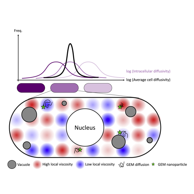
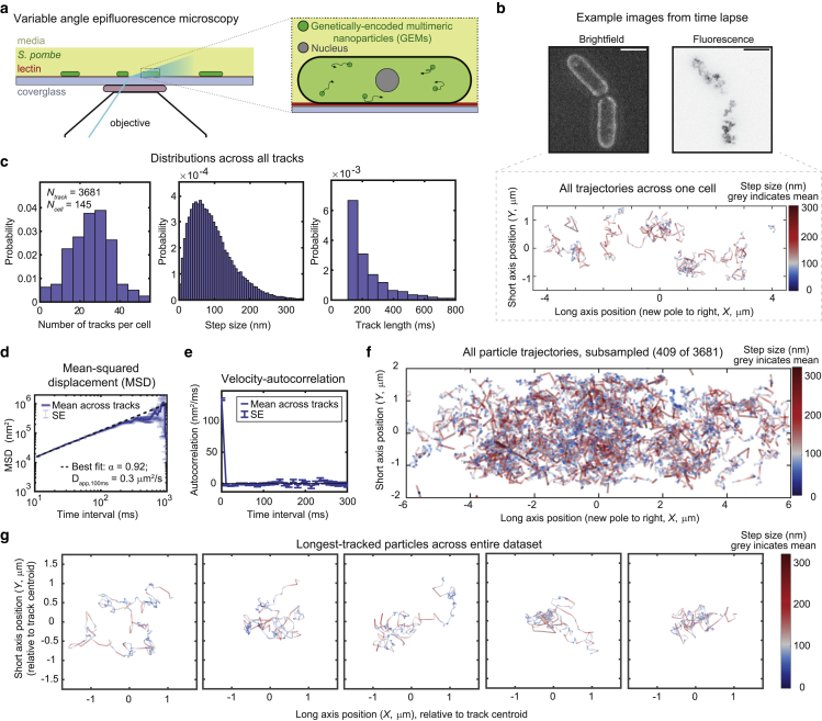
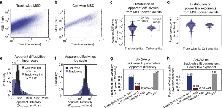
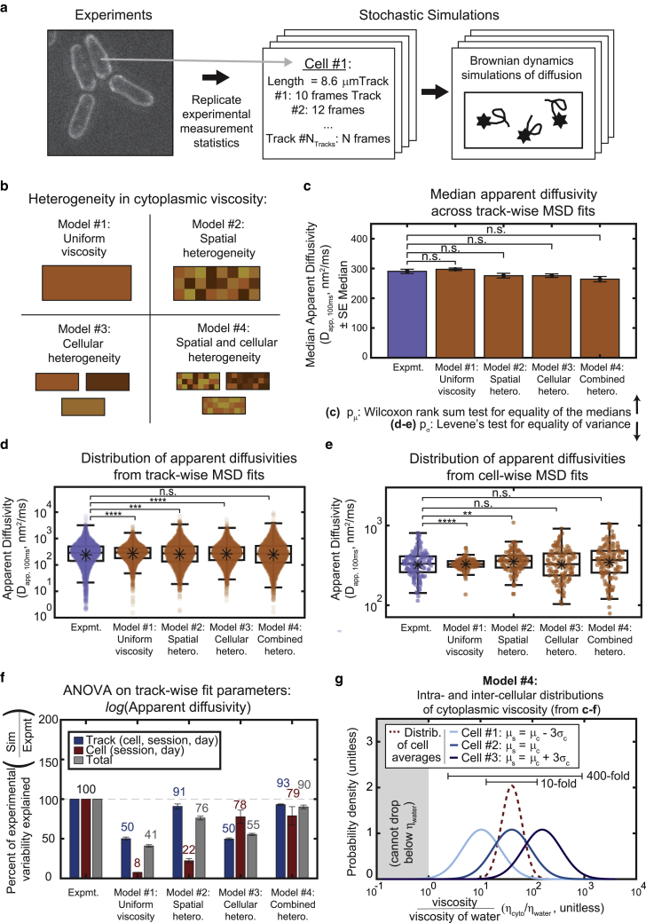
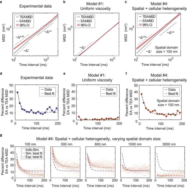
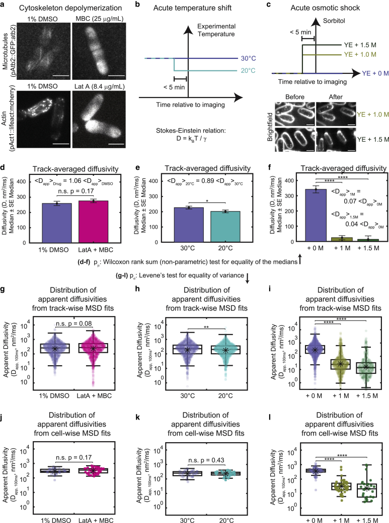
The cytoplasm is a complex, crowded, actively driven environment whose biophysical characteristics modulate critical cellular processes such as cytoskeletal dynamics, phase separation, and stem cell fate. Little is known about the variance in these cytoplasmic properties. Here, we employed particle-tracking nanorheology on genetically encoded multimeric 40 nm nanoparticles (GEMs) to measure diffusion within the cytoplasm of individual fission yeast (Schizosaccharomyces pombe) cellscells. We found that the apparent diffusion coefficients of individual GEM particles varied over a 400-fold range, while the differences in average particle diffusivity among individual cells spanned a 10-fold range. To determine the origin of this heterogeneity, we developed a Doppelgänger simulation approach that uses stochastic simulations of GEM diffusion that replicate the experimental statistics on a particle-by-particle basis, such that each experimental track and cell had a one-to-one correspondence with their simulated counterpart. These simulations showed that the large intra- and inter-cellular variations in diffusivity could not be explained by experimental variability but could only be reproduced with stochastic models that assume a wide intra- and inter-cellular variation in cytoplasmic viscosity. The simulation combining intra- and inter-cellular variation in viscosity also predicted weak nonergodicity in GEM diffusion, consistent with the experimental data. To probe the origin of this variation, we found that the variance in GEM diffusivity was largely independent of factors such as temperature, the actin and microtubule cytoskeletons, cell-cyle stage, and spatial locations, but was magnified by hyperosmotic shocks. Taken together, our results provide a striking demonstration that the cytoplasm is not "well-mixed" but represents a highly heterogeneous environment in which subcellular components at the 40 nm size scale experience dramatically different effective viscosities within an individual cell, as well as in different cells in a genetically identical population. These findings carry significant implications for the origins and regulation of biological noise at cellular and subcellular levels.

Graphical abstract

Figure 1

High-speed particle-tracking nanorheology of GEMs allows detailed statistical analysis of cytoplasmic diffusion. (a) Schematic of the experimental imaging set-up. (b) Example bright-field image (top left) and maximum intensity projection through time of the GEM particle fluorescence (top right) for one representative field of view, alongside the measured nanoparticle trajectories (bottom) for the upper cell in the image. Trajectories are colored by the step size of the particle in nanometers between each time frame of the movie. Gray indicates the mean step size across all tracks in the data set. Scale bar, 5 μm. (c) Histograms of the number of tracks per cell (left), the step size for all time points (middle), and the duration of time that each particle was tracked (right). Note that tracks shorter than 10 time points were not included in the analysis. (d) The mean-squared displacement (MSD) of the particle tracks. The time-averaged MSD was first calculated individually for each track, and then a second averaging was performed to find the (ensemble averaged) MSD across all tracks. Note the logarithmic scale along the x and y axes. (e) The average velocity autocorrelation across all particle tracks. Averaging was performed in the same order as the MSD. (d and e) Error bars represent the standard error (SE). (f) Plots of particle trajectories drawn from many experiments and cells, randomly subsampled for better visibility of individual particle behaviors. Subsampled trajectories include at least one track from 141 of the 145 cells in the data set. Gray indicates the mean step size across all tracks in the data set. (c–f) The data set includes 3681 tracks among 145 cells, recorded from 5 different samples and over 3 different days. (g) Individual trajectory plots for five of the longest-tracked particles (in time), excluding stationary particles. Color scaling of the step size was identical in all panels included in (f and g) (using the mean and SD of the step size across the entire data set).

Figure 2

GEM diffusivity varies over 400-fold across tracks and 10-fold across cells. (a and b) MSDs averaged either (a) by track (averaged over time for each track) or (b) by cell (averaged over time for each track and then averaged across all tracks in each cell). Note the logarithmic scale along the x and y axes. (c and d) Apparent diffusivities (c) and power law exponents (d) calculated from fits of the track-wise and cell-wise MSDs to a power law. Note the logarithmic scale along the y axis. Boxplots: central line, median; gray dot, mean; boxes, 25th and 75th percentiles; whiskers, furthest data points that are not an outlier; outliers, any point that is more than 1.5 times the interquartile-range past the 25th and 75th percentiles. (e and f) The same distributions of the fitted apparent diffusivities plotted in (c), now plotted as a histogram either on a linear scale (e) or on a log scale (f). Probabilities represent the probability density per histogram bin width, such that the sum of the bin heights multiplied by the bin width equals 1. (g and h) Results from a nested ANOVA performed on track-wise fits of diffusivities (g) and power law exponents (h). The amount of the experimentally observed variance that can be explained by track-to-track, cell-to-cell, imaging session-to-session, and day-to-day variability is plotted as a fraction of the total variance. (a–h) The data set is identical to that shown in Fig. 1, c–f, including 3681 tracks among 145 cells, recorded from 5 different samples and over 3 different days.

Figure 3

Stochastic simulations reveal both spatial and cellular heterogeneity in viscosity are required to reproduce the experimentally observed variation. (a) Schematic of the Doppelgänger simulation approach. Each experimentally measured cell and particle were reproduced one-to-one in the simulated data set, with every simulated cell having the same long axis length as its experimentally measured counterpart, and each particle being tracked for the same amount of time. (b) Schematic demonstrating different types of heterogeneity in cytoplasmic viscosity included in each of the four models. Note: the choice of physical domain size for spatial heterogeneity in (c–g) is 1000 nm. (c) Median apparent diffusivity (averaged across all tracks) plotted for the experimental data set as well as each model. Error bars represent the SE of the median. Significance stars represent the result of the Wilcoxon rank sum test for equality of the medians. (d and e) Distributions of apparent diffusivities calculated from fits of the track-wise (d) or cell-wise (e) MSD curves displayed for the experimental data as well as each of the models. Note the logarithmic scale along the y axis. Boxplots are drawn as in Fig. 2. Significance stars represent the result of Levene’s test for equality of variance. (c–e) ^∗p < 0.05, ^∗∗p < 0.01, ^∗∗∗p < 0.001, ^∗∗∗∗p < 0.0001. (f) Results from a nested ANOVA performed on track-wise fits of diffusivities (d). The percent of the experimentally observed cell-to-cell and track-to-track variability that can be explained by each of the models. Bars and error bars represent the mean and the standard error, respectively, across 5 Doppelgänger simulation replicates (g) The distribution of cytoplasmic viscosities, shown relative to the viscosity of water, needed to most closely reproduce the experimental data (i.e., simulations from Model #4, using the same parameters used to generate (c–f)). Histograms are shown for the distribution of average cell viscosities (intercellular heterogeneity, red dashed line) and the distribution of intracellular viscosities for three example cells (blue lines of varying darkness). The examples include a cell whose average viscosity equals that of the cell-wide average (medium blue line), a cell with an average viscosity three SDs above the cell-wide average (dark blue line), and a cell with an average viscosity three SDs below the cell-wide average (light blue line). Note the logarithmic scale along the x axis. The simulation did not allow viscosities below that of water.

Figure 4

Weak nonergodicity of GEM diffusion can be explained by heterogeneity in viscosity. (a) GEM particle MSD versus time, calculated either by ensemble averaging over all particle tracks (EA MSD, red line), or by first time averaging over each track and then ensemble averaging over all particles (TEA MSD, black line). 95% CIs of the EA MSD were calculated by bootstrapping and are plotted as a red shaded region around the EA MSD. Note the logarithmic scale along the x and y axes. (b) The TEA and EA MSD calculated for a representative Doppelgänger simulation for Model #1: uniform viscosity (see Fig. 3b). (c) The TEA and EA MSD calculated for a representative Doppelgänger simulation for Model #4: spatial and cellular heterogeneity in viscosity (see Fig. 3b), using a 100 nm spatial domain size. (d–f) The percent difference between the EA and the TEA MSD ((EA-TEA)^∗100/EA) displayed in (a–c), respectively, plotted as a function of time interval. The best fit of the data to an exponential decay plus a constant: y = Ae^(-Bt)+C is plotted as a thick dashed black line. (g) The percent difference between the EA and TEA MSD for Model #4: spatial and cellular heterogeneity in viscosity, where each subplot represents a different choice for the domain size of the spatial heterogeneity. x and y axes for all subplots are identical. Each light orange line represents an individual simulation, equivalent to the entire experimental data set. Fifty replicate simulations are superimposed onto the plot. Each curve was individually fit to an exponential decay plus a constant: y = Ae^(-Bt)+C, and the best fit parameters were averaged across all 50 simulations to produce the best fit line (thick dashed orange line). The best fit to the experimental data shown in (d) is overlaid as a thick dashed purple line. Of the domain sizes sampled, simulations using the 100 nm domain gives the closest agreement to the experimental data, with the experimental data best fit line lying well within the range of outcomes among replicate simulations. On average, the 100 nm simulation best fit line lies slightly below the experimental best fit line, and the 300 nm simulation best fit line lies slightly above the experimental best fit line. Thus, we estimate the domain size of the cytoplasm is on the order of ∼100–300 nm.

Figure 5

Heterogeneity in cytoplasmic diffusion has varied responsiveness to experimental perturbations. (a) Fluorescence images of fluorescent tubulin (top) and actin (bottom) in the context of the DMSO control (left) and addition of cytoskeleton depolymerizing drugs (right). Scale bars, 5 μm. (b) Schematic of experiments varying the experimental temperature (top) and prediction of the relationships between the diffusivity, D, and the experimental temperature, T, as well as the Boltzmann constant, k_B, and the viscous drag coefficient, ᵞ (bottom). (c) Schematic of experiments varying osmotic shock with sorbitol (top) and example bright-field images of osmotically shocked cells showing a reduction in cell volume (bottom). Scale bars, 5 μm. (d–f) The median diffusivity (bars) and standard error (error bars) are plotted for each experimental condition. Significance stars represent the result of the Wilcoxon rank sum test for equality of the medians. (g–l) Distributions of apparent diffusivities calculated from fits of the track-wise (g–i) or cell-wise (j–l) MSD curves displayed for each condition. Note the logarithmic scale along the y axis. Boxplots are drawn as in Fig. 2. Significance stars represent the result of Levene’s test for equality of variance. (d–l) ^∗p < 0.05, ^∗∗p < 0.01, ^∗∗∗p < 0.001, ^∗∗∗∗p < 0.0001.

References

1. Huang W.Y.C., Yan Q., et al. Groves J.T. Phosphotyrosine-mediated LAT assembly on membranes drives kinetic bifurcation in recruitment dynamics of the Ras activator SOS. Proc. Natl. Acad. Sci. USA. 2016;113:8218–8223. - PMC - PubMed
1. Schmoller K.M. The phenomenology of cell size control. Curr. Opin. Cell Biol. 2017;49:53–58. - PubMed
1. Facchetti G., Knapp B., et al. Howard M. Reassessment of the basis of cell size control based on analysis of cell-to-cell variability. Biophys. J. 2019;117:1728–1738. - PMC - PubMed
1. Patterson J.O., Rees P., Nurse P. Noisy cell-size-correlated expression of cyclin B drives probabilistic cell-size homeostasis in fission yeast. Curr. Biol. 2019;29:1379–1386.e4. - PMC - PubMed
1. Chang A.Y., Marshall W.F. Organelles--understanding noise and heterogeneity in cell biology at an intermediate scale. J. Cell Sci. 2017;130:819–826. - PMC - PubMed
Publication types