Steering particles via micro-actuation of chemical gradients using model predictive control

Abstract

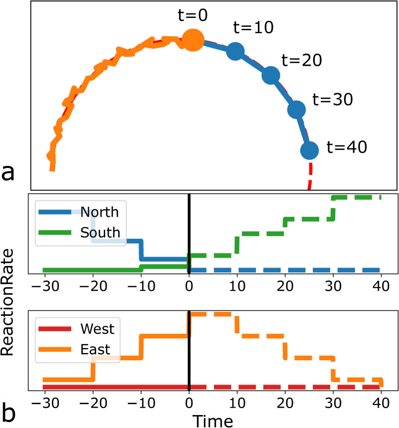
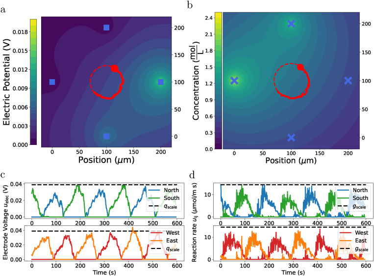
Biological systems rely on chemical gradients to direct motion through both chemotaxis and signaling, but synthetic approaches for doing the same are still relatively naïve. Consequently, we present a novel method for using chemical gradients to manipulate the position and velocity of colloidal particles in a microfluidic device. Specifically, we show that a set of spatially localized chemical reactions that are sufficiently controllable can be used to steer colloidal particles via diffusiophoresis along an arbitrary trajectory. To accomplish this, we develop a control method for steering colloidal particles with chemical gradients using nonlinear model predictive control with a model based on the unsteady Green's function solution of the diffusion equation. We illustrate the effectiveness of our approach using Brownian dynamics simulations that steer single particles along paths, such as circle, square, and figure-eight. We subsequently compare our results with published techniques for steering colloids using electric fields, and we provide an analysis of the physical parameter space where our approach is useful. Based on these findings, we conclude that it is theoretically possible to explicitly steer particles via chemical gradients in a microfluidics paradigm.

FIG. 1.

An example of microfluidic device for steering particles via diffusiophoresis. The trajectory (red line) of a colloidal particle (red circle) is controlled using feedback from a vision system that is fed to a computer algorithm that computes reaction rates for chemical actuators. The chemical gradient of the control area is shown by the contour plot in the lower right, where bright yellow indicates a high-concentration area and dark blue a low one.

FIG. 2.

Domain geometry for (a) electric field and (b) chemical gradient simulations. In (a), electrodes (blue squares) are controlled by changing their voltages with time to move a colloidal particle (orange dot) on a target path. In (b), the electrodes are replaced by chemical reactions (blue x’s). In each, the dashed blue line is the area in which the particle is allowed to move (the control region), and the dashed green box is the boundary of the simulated area (the simulation domain). The electrodes or chemical probes are separated by a distance of $L$, and the simulation domain is a box of side length $3L$.

FIG. 3.

An illustration of how model predictive control steers a colloid on a circular trajectory. (a) The colloid (orange dot) is steered on a reference trajectory (red dashed line) using predictions of its future position (blue dots) with $N_{\mathrm{pred}}$ = 4. In this example, the particle has already been moving for $t=50$ (arbitrary units), and the four future points are predicted at a fixed $\mathrm{\Delta }{t}_{\mathrm{control}}=10$. (b) Past (solid) and predicted (dashed) optimal inputs (i.e., reaction rates) for the four probes located north, south, east, and west of the particle.

FIG. 4.

A comparison between the model velocity from Eq. (21) and the simulated velocity from Eq. (1) (neglecting Brownian motion) for a single impulse of a single probe. The plot uses parameters $\mathrm{\Delta }{t}_{\mathrm{control}}=0.5$ s, $v_0=0.05\mu$m/s, and other parameters as given in Table I. Each velocity is given for both an average particle-probe distance $r=L/2$ (blue lines) and for a large particle-probe distance $r=L$ (green lines). The vertical orange dashed line shows the impact of implementing a cutoff by setting the model velocity to zero after $n_{\mathrm{cutoff}}$ time steps have passed. The portion captured by the dynamic model when the particle is at $L/2$ is shaded in blue, and the portion neglected by the cutoff is shaded in orange.

FIG. 5.

The trajectory and control inputs for both the electric field controller and the chemical gradient controller. (a) An electric field simulation, in which the particle (red dot) is steered to follow a circular trajectory (dashed red line), where the actual path of the particle is shown as a solid red line and the locations of the four electrodes are represented by blue x’s. (b) A chemical simulation, where the four chemical probes are shown as blue x’s. (c) The voltages of each of the four electrodes are shown as a function of time. (d) The chemical reaction rates are shown as a function of time.

FIG. 6.

A particle (red dot) steered on a square-shaped path (red dashed line).

FIG. 7.

A particle (red dot) is steered on a figure-eight path (red dashed line).

FIG. 8.

The model velocity ${\hat{v}}_{\mathrm{diff}}$ from Eq. (24) is shown in blue, along with $t_{\mathrm{s}}$ (red dot) and $N_{\mathrm{pred}}\mathrm{\Delta }{t}_{\mathrm{control}}$ (orange dashed line). The portion of ${\hat{v}}_{\mathrm{diff}}$ captured by the NMPC controller when calculating a future input is shaded in blue, and the remainder is shaded in orange.

FIG. 9.

Plot of the parameter space in terms of speed $v_0$ and length scale $r_d$ of a desired trajectory for a fixed set of system parameters: $L$, $D_s$, and $D_c$ (given in Table I). The region of the parameter space that satisfies the design rules is shaded in blue, while other combinations result in either too much Brownian motion or too slow diffusion. The design rules are defined using $t_{\mathrm{c}}=20T$ and $T=5t_{\mathrm{s}}$. The parameters chosen for the simulations given in Sec. III are represented by a red dot. The minimum length scale predicted by this theory is shown as a gray dot.

FIG. 10.

Plot of the parameter space in terms of speed $v_0$ and length scale $r_d$ of a desired trajectory for three values of the parameter $R_c$. The region of parameter space that satisfies the design rules is located below the green line and above the blue line for a given value or $R_c$.

References

1. Ropp C., Cummins Z., Nah S., Qin S., Seog J. H., Lee S. B., Fourkas J. T., Shapiro B., and Waks E., Nano Lett. 13, 3936 (2013). 10.1021/nl402059u - DOI - PubMed
1. Wu L. Y., Di Carlo D., and Lee L. P., Biomed. Microdevices 10, 197 (2008). 10.1007/s10544-007-9125-8 - DOI - PubMed
1. Mirbagheri M., Adibnia V., Hughes B. R., Waldman S. D., Banquy X., and Hwang D. K., Mater. Horiz. 6, 45 (2019). 10.1039/c8mh00803e - DOI
1. Filippi M., Buchner T., Yasa O., Weirich S., and Katzschmann R. K., Adv. Mater. 34, 2108427 (2022). 10.1002/adma.202108427 - DOI - PubMed
1. Chaudhary S. and Shapiro B., IEEE Trans. Control Syst. Technol. 14, 669 (2006). 10.1109/TCST.2006.876636 - DOI
LinkOut - more resources