[Preprint]. 2023 Jan 26:arXiv:2301.11262v1.

Better than DFA? A Bayesian Method for Estimating the Hurst Exponent in Behavioral Sciences

Affiliations

Better than DFA? A Bayesian Method for Estimating the Hurst Exponent in Behavioral Sciences

Aaron D Likens et al. ArXiv. .

Abstract

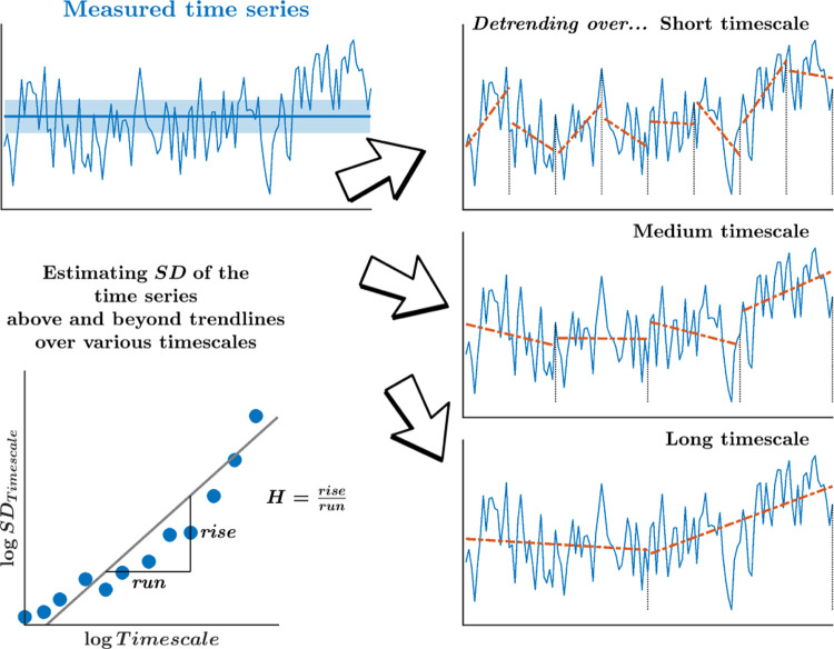
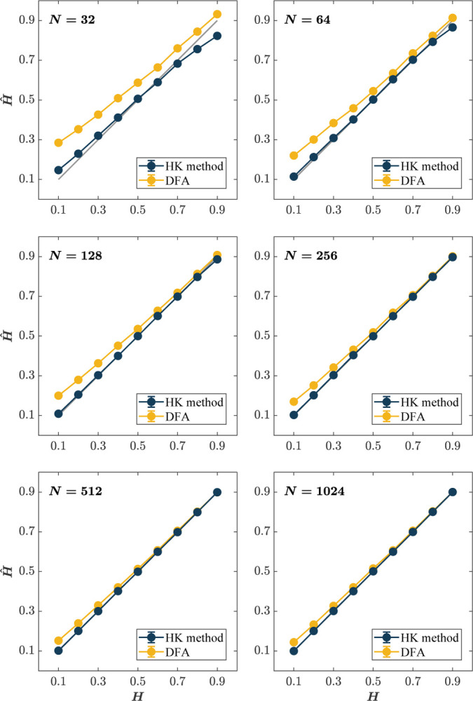
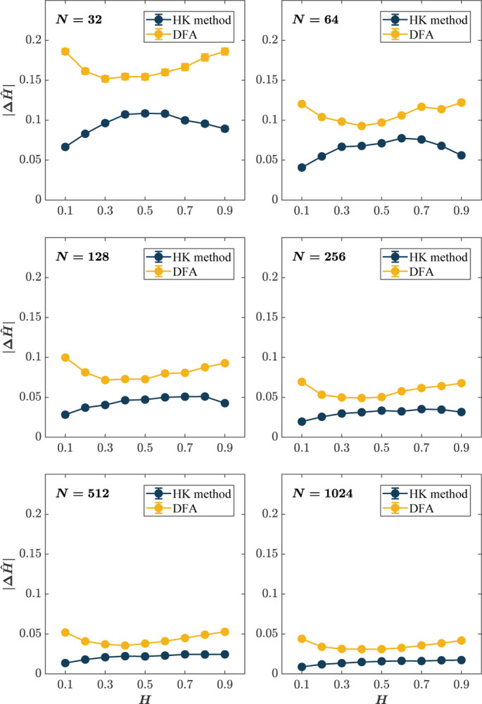
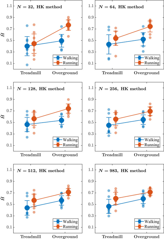
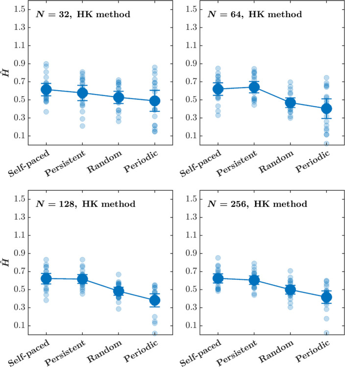
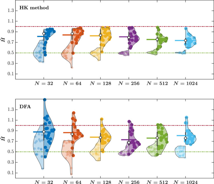
Detrended Fluctuation Analysis (DFA) is the most popular fractal analytical technique used to evaluate the strength of long-range correlations in empirical time series in terms of the Hurst exponent, H. Specifically, DFA quantifies the linear regression slope in log-log coordinates representing the relationship between the time series' variability and the number of timescales over which this variability is computed. We compared the performance of two methods of fractal analysis-the current gold standard, DFA, and a Bayesian method that is not currently well-known in behavioral sciences: the Hurst-Kolmogorov (HK) method-in estimating the Hurst exponent of synthetic and empirical time series. Simulations demonstrate that the HK method consistently outperforms DFA in three important ways. The HK method: (i) accurately assesses long-range correlations when the measurement time series is short, (ii) shows minimal dispersion about the central tendency, and (iii) yields a point estimate that does not depend on the length of the measurement time series or its underlying Hurst exponent. Comparing the two methods using empirical time series from multiple settings further supports these findings. We conclude that applying DFA to synthetic time series and empirical time series during brief trials is unreliable and encourage the systematic application of the HK method to assess the Hurst exponent of empirical time series in behavioral sciences.

Keywords: detrended fluctuation analysis; fractal fluctuations; fractional; human movement; long-range correlation; physiology; variability.


Conflict of interest statement

Declarations. The authors declare no competing financial interests.

Figures

Fig. 1
Fig. 1. Schematic portrayal of the measure of fractality, H, yielded by the DFA.
H relates how the SD-like variation grows across many timescales, statistically encoding how the correlation among sequential measurements might decay slowly across longer separations in time. We use detrending of these variations over progressively longer timescales to remove the mean drift across each of these timescales.
Fig. 2
Fig. 2. The HK method estimates the Hurst exponent, Ĥ, with consistently better accuracy than DFA, which overestimates Ĥ, specifically for short time series and small values of H.
Each panel plots the Mean estimated values of Ĥ for 1, 000 synthetic time series of length N = 32, 64, 128, 256, 512, 1024 with a priori known values of H. The grey line indicates the ideal case where the estimated value is the same as the actual value, i.e., Ĥ = H. Error bars indicate 95% CI across 1000 simulations.
Fig. 3
Fig. 3. Although DFA estimates the Hurst exponent, Ĥ, reasonably accurately for long time series (|ΔĤ| ~ 0.05 for N > 512), the HK method estimates H with consistently better accuracy than DFA.
Each panel plots the Mean absolute error in the estimation of Ĥ, |ΔĤ|, for 1, 000 synthetic time series of length N = 32, 64, 128, 256, 512, 1024 with a priori known values of H. Error bars indicate 95% CI across 1000 simulations.
Fig. 4
Fig. 4. The Hurst exponent, Ĥ, for stride interval time series estimated using the HK method do not depend on the time series length N, but Ĥ estimated using DFA show a strong dependence on N, resulting in larger Ĥ for larger N.
The right and the left violin plots represent the distribution of Ĥ for the original and shuffled stride interval time series, respectively, estimated using the HK method (top) and DFA (bottom). Vertical lines represent the interquartile range of the original Ĥ values, white circles represent the median value of Ĥ, and horizontal lines represent the Mean value of Ĥ for the original stride interval time series. Horizontal dash-dotted green and red lines indicate Ĥ = 0.5 and Ĥ = 1, respectively.
Fig. 5
Fig. 5. The effects of locomotion mode and surface on the Hurst exponent, Ĥ, estimated using the HK method do not depend o such as uniform or truncated Gaussian distributions, etc. the stride interval time series length (see Table 1 for the outcomes of the statistical tests).
Each panel plots the Mean values of Ĥ, estimated using the HK method for stride interval time series of length N = 32, 64, 128, 256, 512, 983. Light blue and light red circles indicate Ĥ values for individual participants in the respective conditions. Error bars indicate 95% CI across 8 participants.
Fig. 6
Fig. 6. The effects of locomotion mode and surface on the Hurst exponent, Ĥ, estimated using DFA wax and wane depending on the stride interval time series length (see Table 2 for the outcomes of the statistical tests).
Each panel plots the Mean values of Ĥ, estimated using DFA for stride interval time series of length N = 32, 64, 128, 256, 512, 983. Light blue and light red circles indicate Ĥ values for individual participants in the respective conditions. Error bars indicate 95% CI across 8 participants.
Fig. 7
Fig. 7. The Hurst exponent, Ĥ, for the finger tapping interval time series estimated using the HK method do not depend on the time series length N, but Ĥ estimated using DFA show a strong dependence on N, resulting in larger Ĥ for smaller and larger N.
The right and the left violin plots represent the distribution of Ĥ for the original and shuffled tapping interval time series, respectively, estimated using the HK method (top) and DFA (bottom). Vertical lines represent the interquartile range of the original Ĥ values, white circles represent the median value of Ĥ, and horizontal lines represent the Mean value of Ĥ for the original stride interval time series. Horizontal dash-dotted green and red lines indicate Ĥ = 0.5 and Ĥ = 1, respectively.
Fig. 8
Fig. 8. The effects of pacing conditions on the Hurst exponent, Ĥ, estimated using the HK method do not depend on the tapping interval time series length (see Table 2 for the outcomes of the statistical tests).
Each panel plots the Mean values of Ĥ, estimated using the HK method for the tapping interval time series of length N = 32, 64, 128, 256, 512, 983. Light blue circles indicate Ĥ values for individual participants. Error bars indicate 95% CI across 19 participants.
Fig. 9
Fig. 9. The effects of pacing condition on the Hurst exponent, Ĥ, estimated using DFA wax and wane depending on the tapping interval time series length (see Table 4 for the outcomes of the statistical tests).
Each panel plots the Mean values of Ĥ, estimated using DFA for the tapping interval time series of length N = 32, 64, 128, 256, 512, 983. Light blue circles indicate Ĥ values for individual participants. Error bars indicate 95% CI across 19 participants.
Fig. 10
Fig. 10. The Hurst exponent, Ĥ, for the response-stimulus interval time series estimated using the HK method do not depend on the time series length N, but Ĥ estimated using DFA show a strong dependence on N, resulting in larger Ĥ for smaller and larger N.
The right and the left violin plots represent the distribution of Ĥ for the original and shuffled response-stimulus interval time series, respectively, estimated using the HK method (top) and DFA (bottom). Vertical lines represent the interquartile range of the original Ĥ values, white circles represent the median value of Ĥ, and horizontal lines represent the Mean value of Ĥ for the original stride interval time series. Horizontal dash-dotted green and red lines indicate Ĥ = 0.5 and Ĥ = 1, respectively.
Fig. 11
Fig. 11. The effects of Task and RSI on the Hurst exponent, Ĥ, estimated using the HK method do not depend on the response-stimulus interval time series length (see Table 5 for the outcomes of the statistical tests).
Each panel plots the Mean values of Ĥ, estimated using the HK method for the response-stimulus interval time series of length N = 32, 64, 128, 256, 512, 1020. Light blue and light red circles indicate Ĥ values for individual participants in the respective conditions. Error bars indicate 95% CI across 6 participants.
Fig. 12
Fig. 12. The effects of Task and RSI on the Hurst exponent, Ĥ, estimated using DFA wax and wane depending on the response-stimulus interval time series length (see Table 6 for the outcomes of the statistical tests).
Each panel plots the Mean values of Ĥ, estimated using DFA for the response-stimulus interval time series of length N = 32, 64, 128, 256, 512, 1020. Light blue and light red circles indicate Ĥ values for individual participants in the respective conditions. Error bars indicate 95% CI across 6 participants.
Fig. 13
Fig. 13. The Hurst exponent, Ĥ, for reaction time series estimated using the HK method do not depend on the time series length N, but Ĥ estimated using DFA show a strong dependence on N, resulting in larger Ĥ for smaller and larger N.
The right and the left violin plots represent the distribution of Ĥ for the original and shuffled stride interval time series, respectively, estimated using the HK method (top) and DFA (bottom). Vertical lines represent the interquartile range of the original Ĥ values, white circles represent the median value of Ĥ, and horizontal lines represent the Mean value of Ĥ for the original stride interval time series. Horizontal dash-dotted green and red lines indicate Ĥ = 0.5 and Ĥ = 1, respectively.
Fig. 14
Fig. 14. The effect of the speaker—human vs. text-to-speech (TTS) synthesizer—on the Hurst exponent, Ĥ, estimated using the HK method and DFA does not depend on the reaction time series length.
Each panel plots the Mean values of Ĥ, estimated using the HK method and DFA for reaction time series of length N = 32, 64, 128, 256, 512, 983. Light blue and light red circles indicate Ĥ values for individual participants in the respective conditions. Error bars indicate 95% CI across 10 participants.

Similar articles

References

    1. Hurst H.E.: Long-term storage capacity of reservoirs. Transactions of the American Society of Civil Engineers 116(1), 770–799 (1951). 10.1061/TACEAT.0006518 - DOI
    1. Mandelbrot B.B., Wallis J.R.: Computer experiments with fractional Gaussian noises: Part 1, averages and variances. Water Resources Research 5(1), 228–241 (1969). 10.1029/WR005i001p00228 - DOI
    1. Beran J., Terrin N.: Estimation of the long-memory parameter, based on a multivariate central limit theorem. Journal of Time Series Analysis 15(3), 269–278 (1994). 10.1111/j.1467-9892.1994.tb00192.x - DOI
    1. Kantelhardt J.W., Berkovits R., Havlin S., Bunde A.: Are the phases in the Anderson model long-range correlated? Physica A: Statistical Mechanics and its Applications 266(1–4), 461–464 (1999). 10.1016/S0378-4371(98)00631-1 - DOI
    1. Efstathiou M., Varotsos C.: On the altitude dependence of the temperature scaling behaviour at the global troposphere. International Journal of Remote Sensing 31(2), 343–349 (2010). 10.1080/01431160902882702 - DOI

Publication types

LinkOut - more resources