Magnon scattering modulated by omnidirectional hopfion motion in antiferromagnets for meta-learning

Abstract

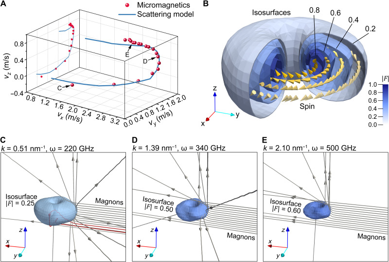
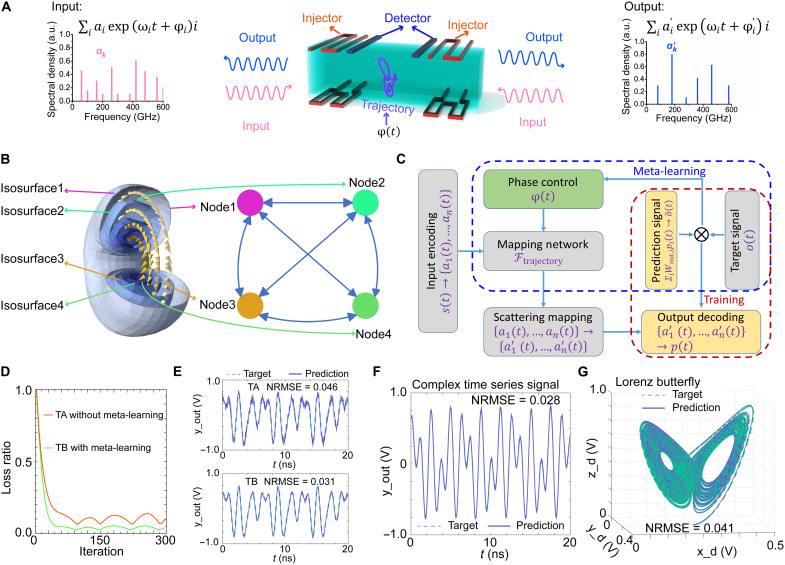
Neuromorphic computing is expected to achieve human-brain performance by reproducing the structure of biological neural systems. However, previous neuromorphic designs based on synapse devices are all unsatisfying for their hardwired network structure and limited connection density, far from their biological counterpart, which has high connection density and the ability of meta-learning. Here, we propose a neural network based on magnon scattering modulated by an omnidirectional mobile hopfion in antiferromagnets. The states of neurons are encoded in the frequency distribution of magnons, and the connections between them are related to the frequency dependence of magnon scattering. Last, by controlling the hopfion's state, we can modulate hyperparameters in our network and realize the first meta-learning device that is verified to be well functioning. It not only breaks the connection density bottleneck but also provides a guideline for future designs of neuromorphic devices.

Fig. 1.. Spin configurations of hopfions in the lowest-energy state.

(A and B) Isosurfaces n_z = 0 of (A) an H-1 hopfion and (B) an H-2 hopfion. The direction of the Neel field is represented by colors in the hue, saturation, and lightness (HSL) color space. The pale green planes are the xy and yz planes. The top left insets are the yz slices of the hopfions, and the bottom right insets are the xy slices of the hopfions. It can be seen from the axis orientation that the H-1 hopfion is oriented toward the $[1\overline{1}1]$ direction, while the H-2 hopfion is oriented toward the [001] direction. (C and D) Preimages of the Neel vectors with xy angles of 0°, 90°, 180°, and 270° for (C) the H-1 hopfion and (D) the H-2 hopfion. The white torus represents the isosurface n_z = 0.

Fig. 2.. Polarization dependence of hopfions’ motion.

(A) Trajectories of H-1 hopfions driven by spin waves with different kinds of polarization incoming along the $[\overline{1}1\overline{1}]$ direction. The spin waves are excited by a time-varying magnetic field of amplitude 2.0 T and a frequency of 440 GHz. (B) Trajectories of H-1 hopfions driven by spin waves with different kinds of polarization incoming along [110]. The spin waves are excited by a magnetic field of amplitude 5.0 T and a frequency of 440 GHz. (C) Displacements of H-2 hopfions driven by spin waves whose phase offset cycles were from 0° to 360° in a step of 30°. The phase offset for each point is represented by a color with a distinctive hue. The Hall plane is highlighted in pale yellow. The spin waves are propagating along [100]. The exciting magnetic field is the same as the one in (B). (D) Geometric picture of polarization dependence. The top shows the mapping from the phase offset to the Hall angle. The red plane denotes the Hall plane. The light cyan cone with its apex at the origin exhibits the area the imaginary displacement may pass through. The yellow vector with a yellow ending point represents the imaginary displacement given the azimuthal angle or, in other words, the phase offset. The actual displacement, represented by a red vector with a red ending point, turns out to be the projection of the imaginary displacement onto the Hall plane. The bottom shows the measured function between the phase offset and tanα_Hall, which is direct evidence for the picture shown in the top.

Fig. 3.. Mechanism for realizing omnidirectional motion of a hopfion in the 3D space.

(A) Proposed experimental setup for omnidirectional motion. The cyan glass is the magnet, in the center of which a violet torus is embedded, representing the hopfion. The red wires are the antennae responsible for inducing exciting magnetic fields from currents. The two antennae above the magnet are used to excite LX waves, while the two below the magnet are used to excite LY waves. The four antennae are distributed on both sides of the magnet and constitute a pair of spin-wave sources. The spin waves are released using sub-terahertz spin oscillators (–48). (B) Non-coplanar Hall planes of the two spin-wave sources. The cyan cones denote the cones of imaginary displacements. The red planes are the Hall planes. (C) Trajectories of hopfions driven by spin waves of different kinds of polarization emanating from each of the two spin-wave sources. These results confirm the prediction in (B).

Fig. 4.. Example trajectories of hopfions and their spin-wave configurations.

(A, C, E, and G) Direction range of velocity the hopfion covers during the motion, which is extended from a circle to the entire unit sphere. The red arrows in (A) and (C) denote the basis of the skew coordinate system. (B, D, F, and H) Complex trajectories that the hopfion moves along, including (B) a circle, (D) a helix, (F) a Chinese knot, and (H) a trefoil knot. These examples are organized in ascending order of complexity. (I) Waveforms of the incident waves applied in (B) (top) and (D) (bottom). Ψ₂ in the two panels is the same, while Ψ₁ in the bottom is an elongated version of Ψ₁ in the top. (J) Direction of the instantaneous velocity for realizing the Chinese knot. (K) Instantaneous velocity for realizing the trefoil knot.

Fig. 5.. Frequency dependence of magnon scattering.

(A) Velocities of hopfions driven by CCW-C waves at different frequencies. The red points denote the values of the velocities obtained from micromagnetic simulation for frequencies from 220 to 560 GHz in a step of 20 GHz. The blue line is the velocity calculated from the magnon-hopfion interaction model. Both of them are projected onto the yz plane to show their relative position from the side view. (B) Emergent magnetic field F of a hopfion. The isosurfaces of ∣F∣ with values of 0.2, 0.4, 0.6, and 0.8 are exhibited in an increasing depth of blue. The direction of F on the equatorial plane in each shell is represented by a chain of yellow cones. (C to E) Paths of certain magnons in the real space for three specifically selected frequencies. The wave number k and the frequency ω are labeled at the top of each figure. The color depth of a isosurface indicates the magnitude of ∣F∣. The magnitude of the field F on these isosurfaces is no more than it is required to reflect all the magnons. The gray trajectories with arrows on them are the paths of magnons, which are scattered by the field. Some of them are painted red to distinguish themselves from their neighbors. The positions of these arrows are a snapshot of all the outgoing magnons at the same simulation time.

Fig. 6.. Meta-learning neural network based on magnon scattering by a hopfion.

(A) Schematic of the meta-learning neuromorphic device. The process of magnon scattering by the hopfion is used to implement the neural network. Carrying the input signal shown in the left frequency spectrum, magnons are injected into the device through the injector antenna. The scattered magnons are received at the detector antenna and are decoded to the right spectrum to obtain the output signal in arbitrary units (a.u.). (B) Correspondence between the neural network nodes and the isosurfaces of the hopfion. The amplitude of magnons of each frequency can be seen as a node in a neural network. The connections between nodes can be treated as the scattering spectrum of magnons. The connections starting from the same node can be seen as an isosurface of the hopfion. (C) Flowchart of the meta-learning framework. The blue dashed circle denotes the meta-learning step, and the red dashed circle denotes the linear regression step. (D) Normalized loss function (loss ratio) convergence curves for the test task. The red line represents the test without meta-learning. The green line represents the test with meta-learning. (E) Prediction result for the test task without and with the multitask training. Normalized root mean square error (NRMSE) is used to estimate the prediction accuracy. (F and G) Our device performs so well in complex time series tasks that the NRMSE reaches 0.028 for (F) the periodic signal and 0.041 for (G) the Lorenz-like chaotic time series.

References

1. R. Friedberg, T. D. Lee, A. Sirlin, Gauge-field non-topological solitons in three space-dimensions (II). Nucl. Phys. B. 115, 32–47 (1976).
1. M. Rho, A. S. Goldhaber, G. E. Brown, Topological soliton bag model for baryons. Phys. Rev. Lett. 51, 747–750 (1983).
1. G. Finocchio, F. Büttner, R. Tomasello, M. Carpentieri, M. Kläui, Magnetic skyrmions: From fundamental to applications. J. Phys. D Appl. Phys. 49, 423001 (2016).
1. A. Fert, V. Cros, J. Sampaio, Skyrmions on the track. Nat. Nanotechnol. 8, 152–156 (2013). - PubMed
1. S. M. Mohseni, S. R. Sani, J. Persson, T. N. A. Nguyen, S. Chung, Y. E. Pogoryelov, P. K. Muduli, E. Iacocca, A. Eklund, R. K. Dumas, S. Bonetti, A. Deac, M. A. Hoefer, J. Åkerman, Spin torque–generated magnetic droplet solitons. Science. 339, 1295–1298 (2013). - PubMed