Approximations of algorithmic and structural complexity validate cognitive-behavioral experimental results

Abstract

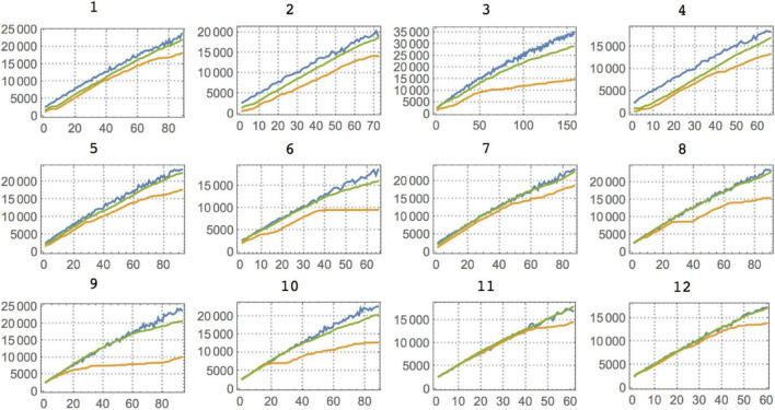
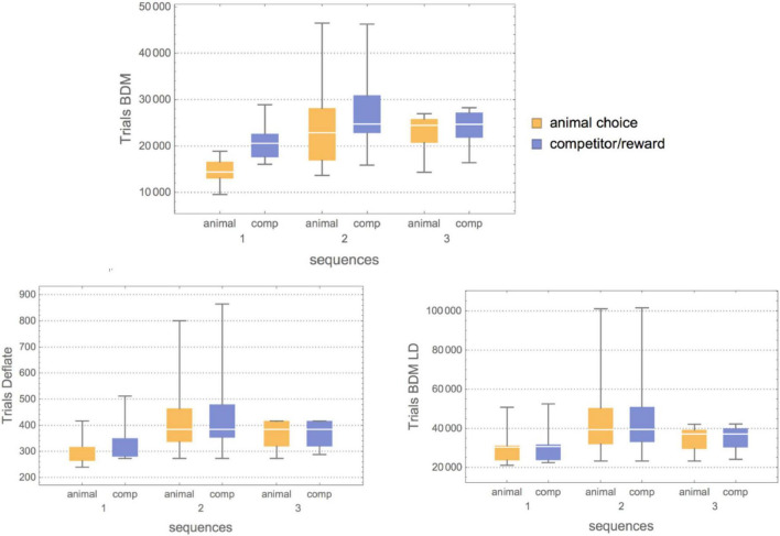
Being able to objectively characterize the intrinsic complexity of behavioral patterns resulting from human or animal decisions is fundamental for deconvolving cognition and designing autonomous artificial intelligence systems. Yet complexity is difficult in practice, particularly when strings are short. By numerically approximating algorithmic (Kolmogorov) complexity (K), we establish an objective tool to characterize behavioral complexity. Next, we approximate structural (Bennett's Logical Depth) complexity (LD) to assess the amount of computation required for generating a behavioral string. We apply our toolbox to three landmark studies of animal behavior of increasing sophistication and degree of environmental influence, including studies of foraging communication by ants, flight patterns of fruit flies, and tactical deception and competition (e.g., predator-prey) strategies. We find that ants harness the environmental condition in their internal decision process, modulating their behavioral complexity accordingly. Our analysis of flight (fruit flies) invalidated the common hypothesis that animals navigating in an environment devoid of stimuli adopt a random strategy. Fruit flies exposed to a featureless environment deviated the most from Levy flight, suggesting an algorithmic bias in their attempt to devise a useful (navigation) strategy. Similarly, a logical depth analysis of rats revealed that the structural complexity of the rat always ends up matching the structural complexity of the competitor, with the rats' behavior simulating algorithmic randomness. Finally, we discuss how experiments on how humans perceive randomness suggest the existence of an algorithmic bias in our reasoning and decision processes, in line with our analysis of the animal experiments. This contrasts with the view of the mind as performing faulty computations when presented with randomized items. In summary, our formal toolbox objectively characterizes external constraints on putative models of the "internal" decision process in humans and animals.

Keywords: Shannon Entropy; ant behavior; behavioral biases; behavioral sequences; communication complexity; tradeoffs of complexity measures.

FIGURE 1

Flow chart of the Coding Theorem Method (CTM) and its implementation Algorithmic Complexity for Short Strings (ACSS), available as a package for the R programming language, shows how K and LD are approximated by way of an Algorithmic Probability-based measure upon application of the algorithmic Coding theorem. The method consists in running an enumeration of Turing machines from smaller to larger (by number of states) and determining whether the machine halts or not for a large set of small Turing machines for which either their halting time can be decided (with the so-called Busy Beaver functions) or an educated theoretical and numerical guess made. The algorithm counts the number of times a sequence is produced, which is a lower bound on its algorithmic probability, and then is transformed to an upper bound of the sequence’s Kolmogorov complexity using the so-called algorithmic Coding theorem (Bottom Left). The same algorithm also finds the shortest, fastest Turing machine that produces the same sequence, hence providing an estimation of its Logical Depth (Bottom Right). An online tool that provides estimations of CTM, and soon will include BDM too, can be found at http://www.complexity-calculator.com.

FIGURE 2

Log correlation between normalized (by a common constant) complexity measures and ant communication time. Kolmogorov complexity (employing an Algorithmic Probability based CTM measure) and Logical Depth (also measured by BDM) display the greatest correlation, with longer times for more complex K and LD. Shannon Entropy and lossless compression display no sensitivity to differences in the sequence. Compress behaves like Entropy.

FIGURE 3

(Top Left) Raw yaw torque series of the three fruit fly groups (about 38,000 data points from a 30-min recorded flying period). (Right Top) Box plot of the series Kolmogorov complexity as measured by CTM over all flies in the three groups (6, 18, and 13). Each replicate was given a different color. (Right) In agreement with the results of Maye et al. (2007) the median complexity of the open-loop group is the most removed from (algorithmic) randomness. The values were normalized by maximum K complexity according to CTM (as compared to the substrings of greatest complexity as calculated from CTM). (Bottom Left) Box plot of the series’ Logical Depth complexity as measured by CTM over all flies in the three groups. The results suggest that the open-loop group has the highest significant median structural complexity (Logical Depth), hence suggesting greater causal history or calculation and a greater remove from randomness. In contrast, the other two groups are closer to pseudo-randomly generated sequences using a log uniform PNRG. This supports the original authors’ findings but adds that uniform stimuli seem to have a lower effect than no stimulus, and that the absence of stimuli also leads to different behavior, perhaps as a strategy to elicit environmental feedback. In both plots, all values were normalized by maximum LD complexity to have them between 0 and 1. In both box plots, the trivial sequences consist of 1 s, and therefore are maximally removed from randomness for Kolmogorov complexity (but are closer to randomness in the LD plot).

FIGURE 4

(Top) The same rat number 6 in the three different environments with different virtual competitors. With Competitor 1 this particular rat shows two kinds of “phase transitions”, leading to a decrease in its behavioral complexity. The standard strategy appears to be to start off by displaying random behavior to test the competitor’s prediction capabilities, switching between different patterns up to a point where the rat settles on a successful strategy that allows it to simply repeat the same behavior and yet receive the maximum reward after fooling the competitor. This phase comes later for Competitor 2 (Bottom Left), given that this new virtual competitor is slightly more sophisticated. For Competitor 3 (Bottom Right), the rat is unable to outsmart it because it implements a more sophisticated predictive algorithm. The rat either cannot settle on a single strategy and keeps performing a random search or decides to switch to or remain in a particular mode after finding itself outsmarted by the virtual competitor.

FIGURE 5

Complexity (BDM) plots for all 12 individuals (rats) against Competitor 1. For Competitors 2 and 3, the most salient feature is that against Competitor 1 the rats show a quick decrease in complexity that allows them to keep the maximal reward (in all three cases. The rats were close to the maximal possible reward except for Competitor 3, where they continued to act randomly, either as a strategy or because they remained in the exploratory transition that is displayed at the beginning of every experiment). Color legends and axis labels are the same as in Figure 4.

FIGURE 6

(Top) Box plots showing the results of three algorithmic information-theoretic complexity measures applied to the behavioral sequences for both animals and competitors (comp) in all three environments of increasing complexity (more powerful virtual competitor predictive capabilities). For BDM (Top), for Competitor 1, the complexity of both the animal and the competitor is low. Still, the gap between medians is extensive, meaning that the animal quickly outsmarted the competitor. For Competitor 2, however, not only is an increase in Kolmogorov complexity shown, but the median gap between the animal’s behavioral complexity and the competitor’s is smaller. Furthermore, the variance is greater, meaning that the animal explored more strategies of different complexity, and finally for Competitor 3 the medians match at higher Kolmogorov complexity (random-looking behavior). (Bottom) Compress (implementing the Deflate lossless compression algorithm) confirmed the BDM results but showed less fine granularity than BDM allowed, likely due to the fact that lossless compression finds it difficult to detect small patterns that both the animals and these simple competitors rely so much upon. BDM LD confirmed the nature of the strategy against Competitor 3, where there is a decrease in structural complexity as compared to the interaction with Competitor 2, hence suggesting that the animal remained in a stochastic mode of low Logical Depth but high Kolmogorov complexity.

References

-
- Bennett C. (1988). “Logical depth and physical complexity,” in The universal turing machine–a half-century survey, ed. Herken R. (Oxford: Oxford University Press; ), 227–257.
- Chaitin G. (1969). On the length of programs for computing finite binary sequences: Statistical considerations. J. ACM 16 145–159. 10.1145/321495.321506 - DOI
LinkOut - more resources
Full Text Sources
Research Materials