A Low-Cost, Low-Power, Multisensory Device and Multivariable Time Series Prediction for Beehive Health Monitoring

Abstract

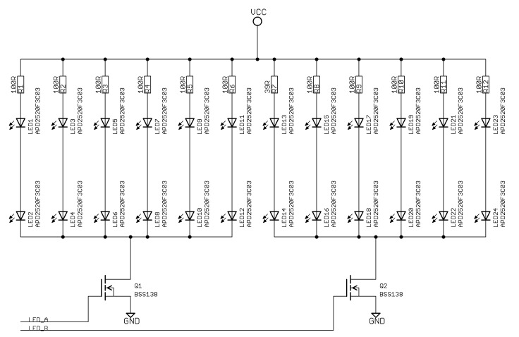
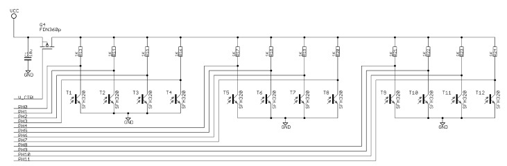
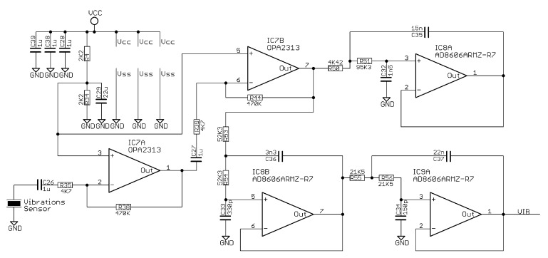
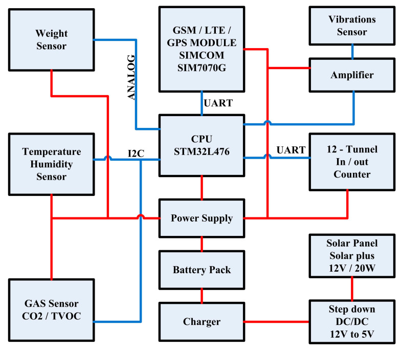
We present a custom platform that integrates data from several sensors measuring synchronously different variables of the beehive and wirelessly transmits all measurements to a cloud server. There is a rich literature on beehive monitoring. The choice of our work is not to use ready platforms such as Arduino and Raspberry Pi and to present a low cost and power solution for long term monitoring. We integrate sensors that are not limited to the typical toolbox of beehive monitoring such as gas, vibrations and bee counters. The synchronous sampling of all sensors every 5 min allows us to form a multivariable time series that serves in two ways: (a) it provides immediate alerting in case a measurement exceeds predefined boundaries that are known to characterize a healthy beehive, and (b) based on historical data predict future levels that are correlated with hive's health. Finally, we demonstrate the benefit of using additional regressors in the prediction of the variables of interest. The database, the code and a video of the vibrational activity of two months are made open to the interested readers.

Keywords: apis mellifera; beehive monitoring; remote sensing; time series prediction.

Figure A1

The bee counter stage processor. It is based on Texas Instruments’ MSP430F5438A microcontroller. The LED_A output activates the LEDs located on the outside of the counter and the LED_B activates the LEDs located on the inner side of the counter. PH 0–PH11 signals are the outputs of phototransistors and through them, in combination with active LEDs, the processor recognizes there is a bee in the tunnel and whether it enters or exits.

Figure A2

Schematic diagram of the LEDs mounted in the tunnels. When Q1 is activated, then the input LEDs emit while when Q2 is activated the output LEDs emit. By sampling at 1KHz, each set emits for 40 uSec each mSec. The total emission time for each sampling cycle is 40 uSec + 40 uSec = 80 uSec. The duty cycle is 8%.

Figure A3

Schematic diagram of phototransistors that detect whether the infrared optical beam of the LEDs has been interrupted. In combination with active LEDs, the processor recognizes the presence or not of a bee and its direction. The Q4 controls the power supply to the circuit and is inactive for as long as it is not needed. At 1 kHz sampling, it is active 80 uSec every 1 mSec. The duty cycle is 8%.

Figure A4

The schematic diagram of the main board of the system. It is based on the STM32L476RG microcontroller of the ST. The system is powered by a battery and the voltage stabilization at 3.3 V is done with the regulator TPS78033022 of Texas Instruments. Communication with the CO₂/Temperature/Humidity sensor board is via the CON3 connector and the data is transferred via I2C Bus. It also has an SD card with power control to minimize consumption when not in use. Communication with the bee counter is via serial communication (UART) via connector SV3. The weight sensor amplifier is connected to connector SV2, the analog output of which drives channel 16 of the ADC. The recording of micro-vibrations is done through analog input (signal VIB, CH15 of ADC) in a file.mp3.

Figure A5

Electronic circuit of the air quality sensors (CCS811 of BioSense company) and temperature-humidity (SHT31 of Sensirion company). Communication with the main processor occurs via I2C Bus.

Figure A6

Electronic amplifier circuit of the weight sensor. It accepts input from the weight sensor and gives a voltage that is proportional to the weight. Voltage to weight conversion is performed on the system processor.

Figure A7

The schematic diagram of the communication circuit. It is based on simcom’s SIM7070G Cat-M/NB LTE GSM module. It connects via a UART port to the main processor and sends the data to the server with a POST request.

Figure A8

The schematic of the piezoelectric sensor amplifier. Amplifies the sensor’s output voltage microvariations (BeStar FT-35T-2.6A1), filtered with a 4KHz low pass filter whose output leads the analog input to the processor.

Figure A9

The schematic diagram of the charging circuit. It is based on Texas Instruments’ BQ24075 integrated circuit. It accepts input from the photovoltaic via DC/DC converter so that it does not exceed 5V. It has a connection input for the battery, and the output (VBATT) provides power to the system when there is a charge on the battery and/or when there is sunshine.

Figure 1

(a) beehives monitored in the course of this work with a number of sensors. The e-beehive in the field. (b) an observation beehive allows us to spot the queen and observe the patterns of activity inside it.

Figure 2

Block diagram of the e-beehive’s multichannel recorder. The system is controlled by an STM32L476RG ARM CPU of ST that simultaneously picks up the vibrations, the bee traffic in the entrance, the gas sensors (CO₂, TVOC), the environmental variables, the vibrations and the measurements of a weight scale. All recordings, are stored in the SD card and transmitted through the LTE module. The device is powered by a 20 W solar panel that charges a battery pack of 12,000 mAh.

Figure 3

(a): the central monitoring unit in the center of the picture with some of the sensing modalities attached. All sensors are sampled simultaneously, and their readings are collected from the main CPU. (b): a closer look at the electronics board prototype. One can discern the CPU in the center, the GPU and communications modem on top, the SD card on top right, the battery on the bottom that connects to the solar panel.

Figure 4

A part of the multivariable time series. Forming sensory data this way allows better forecasts due to complementarity of informational queues.

Figure 5

Cross correlation heatmap of all sensory inputs. TVOC and CO₂ show high correlation and humidity and temperature strong anti-correlation. In and out counts are highly correlated.

Figure 6

Daily balance of power consumption using a 20 W solar panel. Note, the sufficiency of the power-supply scheme, even in winter time, for hourly emissions of data.

Figure 7

(a): boxplots pinpoint outliers in the recordings of CO₂ concentration. They also show most probable value of concentration and the spread of values. (b): descriptive statistics: the mean value, the spread denoted by std (standard deviation), the min and max values are of special importance to the interpretation of the data.

Figure 8

(a) boxplots pinpoint the outlier value of >8000 in the recordings of the TVOC. (b) TVOCs have a smaller spread and lower values compared to CO₂.

Figure 9

(a) the bees covering the gas sensor with propolis on the left. We left only partial coverage as it was totally covered. (b) new, gas-penetrated box houses the gas sensor and placed in the beehive in such a way that not all sides can be covered by propolis.

Figure 10

(a) boxplots pinpoint outliers in the recordings of temperature (°C) that are deemed dangerous for the health of the beehive if they are prolonged. This is not the case here. (b) mean, std, min and max values are valuable to look out for normal values for temperature fluctuations and outliers.

Figure 11

(a) boxplots pinpoint outliers in the recordings of humidity. Beehives must not have measurement near 90% RH for a long time as this implies condensation. (b) the mean and std values show that the humidity levels are normal inside the hive. Special attention should be given to the 90% RH that is, however, a non-persisting outlier.

Figure 12

Descriptors of energy bands. The spectrogram is a time-frequency 2D representation in dB. The descriptors are summing the energy in the corresponding bands 0–100Hz, 200–350 Hz, 300–450 Hz, 400–600 Hz.

Figure 13

Vibrational signals taken from a piezoelectric transducer from within a hive with several thousand bees. (a) a morning recording. (b) an evening recording.

Figure 14

MAPE over a horizon of 1 day (5 min × 12 × 24 data points to be predicted) in the humidity variable.

Figure 15

Prediction of humidity inside the hive on the whole dataset. Prediction starts after ’04–December–2022’. In red, the actual values and in blue the prediction and the uncertainty intervals.

Figure 16

Prophet: prediction of humidity inside the hive. Zooming in the test period.

Figure 17

Decomposing the time series in trend (a) and cyclicity factors (b,c). Practically, no weekly trend is detected in (b), and a daily strong cyclicity of humidity detected between day and night hours in (c). In (d) the role of extra regressors is quantified.

Figure 18

Correlation of features. The hour feature affects CO₂, TVOC, TEMP and strongly the bee traffic in the entrance. The day_of_the_year variable affects weight. CO₂ and TVOC are highly correlated and in and out bee counts as well.

Figure 19

Feature importance on the regression task of forecasting the humidity level inside the beehive using gradient boosting trees (XGBoost).

Figure 20

Prediction of humidity inside the hive using gradient boosted decision trees. Zooming in the test period.

References

1. Watson K., Stallins A. Honey Bees and Colony Collapse Disorder: A Pluralistic Reframing. Geogr. Compass. 2016;10:222–236. doi: 10.1111/gec3.12266. - DOI
1. [(accessed on 10 January 2023)]. Available online: https://ec.europa.eu/commission/presscorner/detail/en/IP_19_6777.
1. Gallai N., Salles J.-M., Settele J., Vaissière B.E. Economic valuation of the vulnerability of world agriculture confronted with pollinator decline. Ecol. Econ. 2009;68:810–821. doi: 10.1016/j.ecolecon.2008.06.014. - DOI
1. Klein A.-M., Vaissière B.E., Cane J.H., Steffan-Dewenter I., Cunningham S.A., Kremen C., Tscharntke T. Importance of pollinators in changing landscapes for world crops. Proc. R. Soc. B. 2006;274:303–313. doi: 10.1098/rspb.2006.3721. - DOI - PMC - PubMed
1. Potts S.G., Biesmeijer J.C., Kremen C., Neumann P., Schweiger O., Kunin W.E. Global Pollinator Declines: Trends, Impacts and Drivers. Trends Ecol. Evol. 2010;30:1–9. doi: 10.1016/j.tree.2010.01.007. - DOI - PubMed