Subspace orthogonalization as a mechanism for binding values to space

Abstract

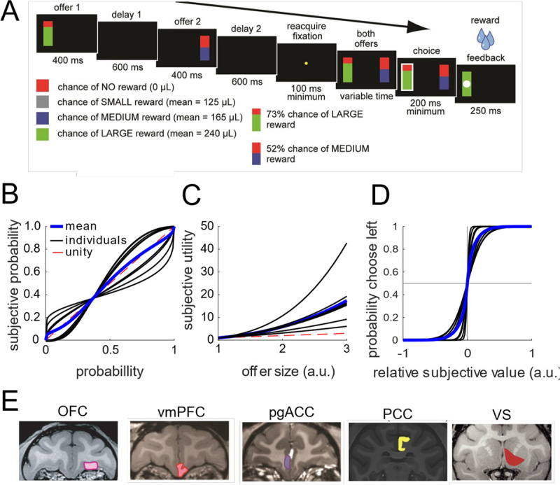
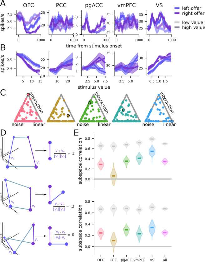
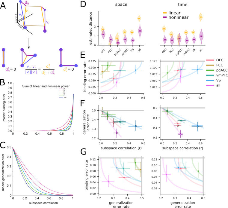
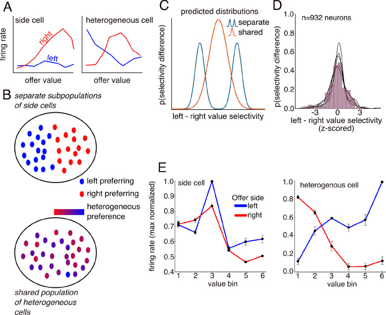
When choosing between options, we must solve an important binding problem. The values of the options must be associated with information about the action needed to select them. We hypothesize that the brain solves this binding problem through use of distinct population subspaces. To test this hypothesis, we examined the responses of single neurons in five reward-sensitive regions in rhesus macaques performing a risky choice task. In all areas, neurons encoded the value of the offers presented on both the left and the right side of the display in semi-orthogonal subspaces, which served to bind the values of the two offers to their positions in space. Supporting the idea that this orthogonalization is functionally meaningful, we observed a session-to-session covariation between choice behavior and the orthogonalization of the two value subspaces: trials with less orthogonalized subspaces were associated with greater likelihood of choosing the less valued option. Further inspection revealed that these semi-orthogonal subspaces arose from a combination of linear and nonlinear mixed selectivity in the neural population. We show this combination of selectivity balances reliable binding with an ability to generalize value across different spatial locations. These results support the hypothesis that semi-orthogonal subspaces support reliable binding, which is essential to flexible behavior in the face of multiple options.

Figure 1.

Task outline and brain areas. A. The risky-choice task is a sequential offer decision-task that we have used in several previous studies (e.g., Strait et al., 2014). In the first 400 ms, subjects see the first offer as a bar presented on either the left or right side. The above shows an example on the left. This offer is followed by a 600 ms delay, a 400 ms offer 2 window, another delay (2) window, and then choice. The full task involved either small, medium or large reward offers. The small reward trials were actually those with safe (guaranteed) offers. We only analyzed the risky choice trials, which were those including the medium and large reward. B-D. From left to right, the plots show for all subjects the model fitted (left) subjective probability, (middle) subjective utility, and (right) relative subjective value choice curves. E. MRI coronal slices showing the 6 different core reward regions that were analyzed.

Figure 2.

Example neurons, model comparison, and subspace correlations. A. The firing rates of example neurons from each region during the offer window, shown for high and low value offers presented on the left or right side (100 ms boxcar filter, shaded area is SEM). B. The value-response function for each neuron in A. The value-response function fit by the linear regression model with an interaction term is overlaid (dashed lines). C. A simplex showing the weight given to each of the noise-only, linear, and interaction regression models by the Bayesian model stacking analysis. The points corresponding to the example neurons shown in A and B have dark outlines here. Both the linear and interaction categories include both linear and spline value representation models. D. Schematic of three different representational geometries that would lead to different subspace correlation results. (top) Two perfectly aligned value vectors v_l and v_r in population space (left) would produce a subspace correlation close to 1 (right). (middle) Two partially aligned value vectors v_l and v_r in would produce a subspace correlation between 0 and 1 (note there is an additional possibility: partially aligned but negatively correlated subspaces; not schematized). (bottom) Two unaligned value vectors v_l and v_r would produce a subspace correlation close to 0. E. Subspace correlations for all regions for the offer presentation window. The gray point is the subspace correlation expected if the left- and right value subspaces were aligned and corrupted only due to noise. E. Same as D. for the delay period.

Figure 3.

Formalizing subspace structure through a geometric theory of binding and generalization for neural codes. A. Schematic of the geometric decomposition. (top) The representation from Figure 2 is decomposed into linear d_L (yellow) and nonlinear d_N (purple) components. (bottom) The relative length of these components determines the subspace correlation from before: d_N = 0 and d_L > 0 implies perfect subspace correlation (bottom left), both d_N > 0 and d_L > 0 implies intermediate subspace correlation (bottom middle), and d_N > 0 while d_L = 0 implies zero subspace correlation (bottom right). B. The relationship of the binding error rate predicted by our theory with subspace correlation. The different lines are codes with different sums of squared linear and nonlinear distances. The line is created by varying the tradeoff between linear and nonlinear distance such that the sum remains constant. The left side of the line is when linear distance is zero and nonlinear distance is the total distance; the right side is the opposite extreme. C. The same as B but for the generalization error rate. D. (left) The nonlinear and linear distances estimated for the left and right value codes within each brain region. (right) The same as on the left, but for the offer 1 and offer 2 value codes. The violin plot shows the distribution of bootstrap resamples. E. The predicted binding error rate as a function of subspace correlation for each region, derived from the distance estimates in D. The left-right plot convention is the same as in D. The gray line shows the chance level of binding errors. F. The predicted generalization error rate as a function of subspace correlation for each region, derived from the distance estimates in D (for the open circles) and computed empirically with a linear decoder (for the outlined circles). The gray line is the chance level. The left-right plot convention is the same as in D. G. Each region shown on the plane defined by the generalization and binding error plane, derived from the distance estimates in D. The gray lines are the chance levels for each of the error types. The left-right plot convention is the same as in D.

Figure 4.

Understanding the nonlinear selectivity underlying subspaces and binding. A. Two schematic kinds of nonlinear selectivity: (left) A strong side preference and (right) two different response profiles to the two different sides. B. The two kinds of selectivity give rise to two distinct hypotheses for selectivity across the population: (top) Separate subpopulations, each composed of cells with a strong preference for one of the two positions and (bottom) a single population composed of cells with heterogeneous response profiles for the two sides. Both forms of nonlinear population selectivity achieve subspace binding. (C). These hypotheses (A-B) predict differences in how the distribution of selectivity differences for left and right value subspaces will appear. The separate subpopulations hypothesis predicts a closer to bimodal distribution (blue line), while the shared, heterogeneous hypothesis predicts a unimodal distribution (orange line). (D) estimated distribution of differences in value selectivity for left and right subspaces for offer 1 on time window. Each line is a different region, showing they are all unimodal. (E). Example OFC nonlinear encoding neurons showing: one has a weak side preference (left) and the other has a heterogeneous response profile (right).

References

1. Babadi B., & Sompolinsky H. (2014). Sparseness and expansion in sensory representations. Neuron, 83(5), 1213–1226. - PubMed
1. Barak O., Rigotti M., & Fusi S. (2013). The sparseness of mixed selectivity neurons controls the generalization–discrimination trade-off. Journal of Neuroscience, 33(9), 3844–3856. - PMC - PubMed
1. Bays P., Schneegans S., Ma W. J., & Brady T. (2022). Representation and computation in working memory. psyRxiv preprint: 10.31234/osf.io/kubr9 - DOI - PubMed
1. Bernardi S., Benna M. K., Rigotti M., Munuera J., Fusi S., & Salzman C. D. (2020). The geometry of abstraction in the hippocampus and prefrontal cortex. Cell, 183(4), 954–967. - PMC - PubMed
1. Blanchard T. C., Piantadosi S. T., & Hayden B. Y. (2018). Robust mixture modeling reveals category-free selectivity in reward region neuronal ensembles. Journal of neurophysiology, 119(4), 1305–1318. - PMC - PubMed
Publication types
LinkOut - more resources