Multiplexed Subspaces Route Neural Activity Across Brain-wide Networks

Abstract

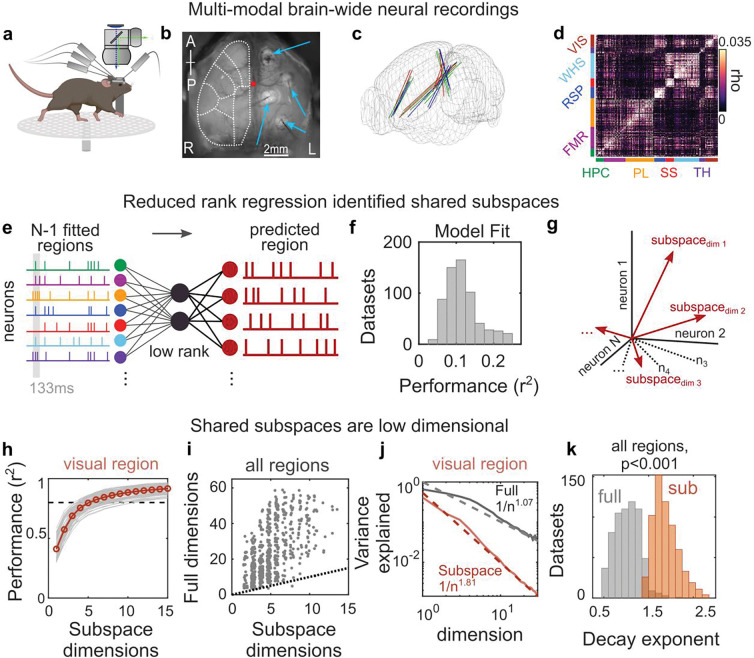
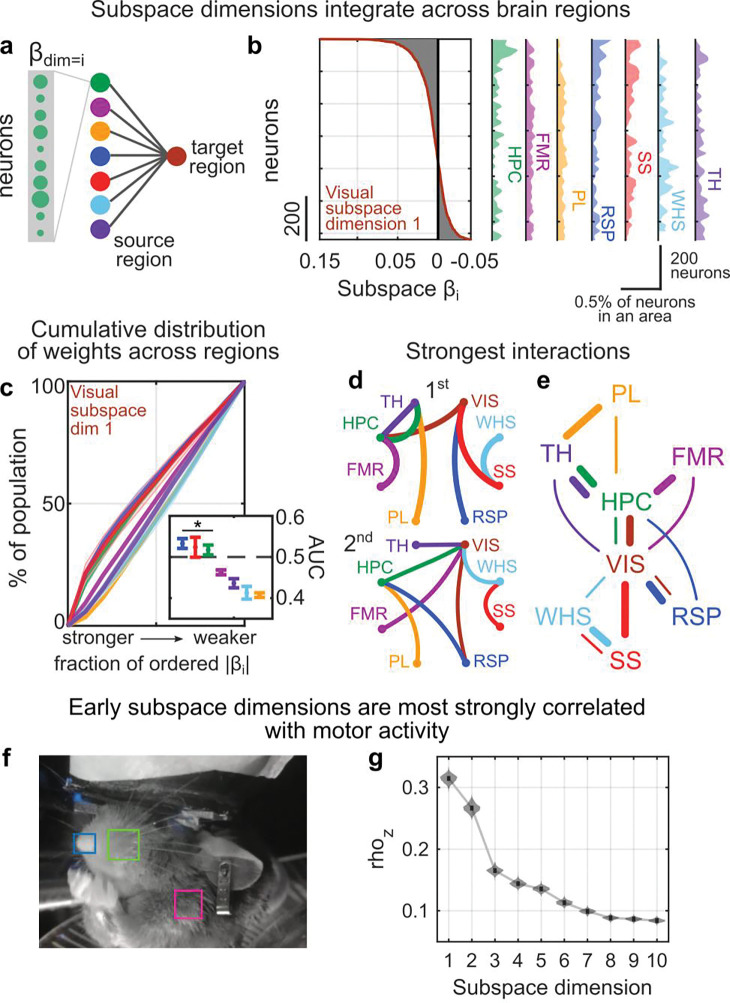
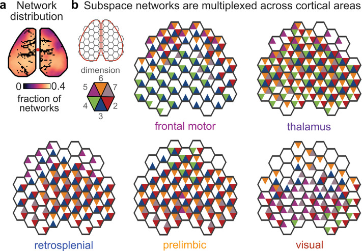
Cognition is flexible. Behaviors can change on a moment-by-moment basis. Such flexibility is thought to rely on the brain's ability to route information through different networks of brain regions in order to support different cognitive computations. However, the mechanisms that determine which network of brain regions is engaged are unknown. To address this, we combined cortex-wide calcium imaging with high-density electrophysiological recordings in eight cortical and subcortical regions of mice. Different dimensions within the population activity of each brain region were functionally connected with different cortex-wide 'subspace networks' of regions. These subspace networks were multiplexed, allowing a brain region to simultaneously interact with multiple independent, yet overlapping, networks. Alignment of neural activity within a region to a specific subspace network dimension predicted how neural activity propagated between regions. Thus, changing the geometry of the neural representation within a brain region could be a mechanism to selectively engage different brain-wide networks to support cognitive flexibility.

Figure 1.. Interactions between brain regions are organized into subspaces.

(a) Schematic of experiments combining neural recordings from four Neuropixels probes across cortical and subcortical regions and simultaneous widefield calcium imaging of neural activity across dorsal cortex. (b) Field of view of widefield imaging showing the dorsal cortex and four craniotomies with implanted electrodes (thin gray shadows; indicated by blue arrows). Dotted white lines outline general cortical regions (see Fig. S1 for parcellation). R and L denote animal’s right and left. (c) Reconstructed probe locations from six recordings in three mice; colors indicate mice. (d) Correlogram showing correlation between pairs of cells within a brain region compared to pairs across regions for an example recording. Color bars along axes correspond to brain regions, held constant throughout figures. (e) Schematic of reduced rank regression to predict activity of each neural population. Spontaneous spiking activity was binned to 133ms windows, and the evoked response was removed (see methods). The moment-to-moment spiking variability of one region was predicted using spiking variability of all other regions. (f) Cross-validated predictive performance of all regression models (models fit to n=630 datasets, see methods). (g) Schematic of the shared subspace, showing that the subspace is spanned by a set of dimensions within the neural activity of the predicted region that are correlated with neural activity in other regions. (h-i) A small subspace of neural activity within a region was shared with other regions. (h) Gray lines show cumulative percent of the explainable variance captured by each dimension of the reduced rank regression model (see methods). Red line shows mean performance. Gray lines show cross-validated performance from n=84 datasets. Black dotted line shows 80% of explainable variance. (i) Comparison between the number of subspace dimensions and the number of ‘local’ dimensions needed to explain 80% of the explainable variance within a region. Local dimensionality was estimated with a cross-validated measure, which revealed that 24.1 dimensions (CI: 23.0–25.4) were needed to capture 80% of the explainable variance within each region. Dots show individual datasets (n=630). Dotted line shows unity. (j) Example results from visual cortex comparing the decay in the variance explained by each additional subspace or local dimension. Solid line and shaded regions show mean and SE, respectively (n=84 model fits). Dotted lines show fit of power law. (k) Histogram of power law exponents from fits to full (grey) and subspace (red) dimensionality across all regions (n=630 datasets).

Figure 2.. Subspaces between areas reflect brain-wide networks.

(a) Contributions of neurons in a source region to predicting activity of a target region are given by their beta weights in the regression model. (b) Example distribution of beta weights (x-axis) across all neurons (y-axis) contributing to predicting activity along the first dimension of the shared subspace in visual cortex. Left plot shows distribution across all regions. Right plots show density histogram of weights within each region (normalized to account for different numbers of neurons). (c) Cumulative distribution of the percent of neurons within a source area contributing to the beta weights along the first dimension of the visual subspace (as in panel b). Weights are ordered from strongest to weakest. Lines show mean, shaded region shows bootstrapped 95% confidence interval from n=84 datasets (see methods). Inset shows the mean and confidence intervals of the area under the curve (AUC) for the contributions from each region. Asterix denotes significance at p<0.05 versus an AUC of 0.5, bootstrap test, n=1000 permutations. (d) Schematic showing the network of strongest (top) and second strongest (bottom) interactions between areas, across all datasets. Strength of contributions were taken as the AUC of beta weights (as in panel c, except averaged across all subspace dimensions). Colored lines indicate the subspace target region, i.e., the strongest contribution to FMR is from HPC (pink line). (e) Network graph showing the two strongest interactions between brain areas. Thicker/thinner lines show the first/second strongest interaction, respectively. (f) The relationship between subspace activity and motor activity was quantified by correlating the activity along each subspace dimension with the motion energy of animals’ nose (blue), whisker-pad (green), and shoulder (pink; see methods). (g) Bootstrapped distribution showing the average correlation (y-axis, z-transformed) between motor activity and activity along each subspace dimension (x-axis) across datasets. Subspace dimension 1 was significantly more correlated with motor activity than all other dimensions (p<0.001, n=1000 bootstraps from n=630 datasets).

Figure 3.. Subspaces engage independent but overlapping cortical networks.

(a) Electrophysiology was combined with simultaneous widefield calcium imaging of population-level neural activity across cortex. Variance in neural activity projected along each subspace dimension was correlated with imaging signal to identify the subspace-associated cortical networks. To better match the time constants of imaging and electrophysiology, we used a feedforward neural network to estimate the neural activity underlying the imaged calcium signal (see methods). (b) Representative cortical maps for different dimensions of subspaces from an example dataset. Rows are different regions. Numbers indicate the subspace dimension corresponding to each map. Colored circles around numbers indicate cluster identity of subspace networks. Color intensity of map indicates the strength of correlation between fluorescence activity at that pixel and the spiking activity along a given subspace (see methods). Transparency (alpha) of color is thresholded at significance such that non-significant pixels are more transparent. For visualization, color is scaled independently for first network versus subsequent networks. (c) Similarity of cortical networks. Similarity (x-axis) was computed as the percentage of overlap in significant pixels between cortical maps across all subspace dimensions for a region (see methods). Y-axis shows the fraction of all compared subspaces. Gray bars show all data (across regions, n=630 dataset). Colored lines show mean distribution of each brain region (n=8) across datasets.

Figure 4.. Cortex-wide subspace networks are multiplexed.

(a) Subspace networks uniformly involved regions across cortex. Map shows the average fraction of subspace networks that were significantly correlated with each pixel (out of 10 possible maps per subspace, averaged across datasets from all target regions, n=630). (b) Honeycomb plots showing multiplexing of subspace networks across cortical areas. Each hexagon shows the dimensions of a subspace that significantly engaged over 25% of pixels within that hexagonal parcel of the cortical surface. For visualization, only a subset of dimensions (2–7) is shown.

Figure 5.. Neural responses are aligned to the shared subspace between two regions when those regions are engaged.

(a) Left plots show pattern of cortical fluorescent activity during motif A (top) and motif B (bottom). Right plots show the neural response in whisker (WHS), somatosensory (SS), and retrosplenial (RSP) cortex (from electrophysiological recordings) during each motif. Dot and error bars indicate mean and standard error of baseline-normalized spiking activity across neurons during each motif for an example recording (SS, n=29; WHS, n=230; RSP, n=190 neurons, see methods). (b) Average projection of neural activity in three-region neural space during motif A (red) and B (blue). Neural activity was projected along the first principal component (PC) of the evoked neural responses in each region (see methods). Arrows show evolution of neural activity over time following onset of each motif (motif A, n=336 occurrences; B, n=266; 133ms timesteps). Top inset shows planes fit to this PC space projection. Bottom inset shows bootstrapped distribution of angle between projection of activity (n=1000 bootstraps across motif occurrences). (c) Schematic of proposed mechanism wherein aligning an evoked response to a subspace dimension propagates activity along the associated subspace network. (d) Small rotations in the neural representation can lead to large changes in the projection of the neural response along the subspace. Top plot shows a relatively small change in the alignment between the local representation of activity in somatosensory cortex (taken as the first PC) and the SS-WHS subspace dimension when comparing motif B (blue) to motif A (red; taken from example dataset). Bottom plot shows this translates into a large change in the evoked response along the SS-WHS subspace. The efficacy of the evoked response is measured as the angle between the projection along the SS-WHS subspace and the first PC of the local response within somatosensory cortex. Dotted line indicates 45 degrees (i.e., perfect alignment). (e) Projection of neural activity during both motifs along the first principal component of activity in SS (x-axis) and the first SS-WHS subspace dimension (y-axis). Greater alignment between the two projections was associated with a larger evoked response; the domain and range of which is shown by red and blue lines along axes. Points show timepoints of evoked response during each motif (as in b). Line and shaded region show least squares fit and 95% confidence bounds, respectively.

Figure 6.. Neural responses were aligned to shared subspaces across regions, motifs, and recordings.

(a) Bootstrapped distribution of the average alignment between the evoked neural response in either SS, WHS, or RSP (denoted in bold) during motif A or B and the subspace between that region and another region (see methods). Lower angles (y-axis) reflect stronger alignment. n=1000 paired bootstraps. Panels a-f reflect data from the same example recording. (b) Distribution of average difference in alignment angle between motif A and B across recordings for SS, WHS, and RSP (n=16 comparisons). Difference in angle was computed relative to the motif with greater engagement of a target brain region, i.e., motif A minus B for comparisons involving SS, but motif B minus A for comparisons involving RSP. Thus, negative values indicate that the motif with greater engagement exhibited better alignment between local neural activity and subspace activity. Vertical red lines show mean (solid) and 95% CI of mean (dashed). (c) Bootstrapped distribution of difference in alignment from multiple pairs of motifs and trios of brain regions across recordings (see Fig. S14). Orange violin shows the overall alignment across all comparisons (240 alignment comparisons, see Methods). Overall, the local neural representation and the associated subspace dimension were more aligned when the stronger motif was engaged (p<0.001). Gray violins show alignment distribution for example pairs of motifs/trios of regions (n=32–48 comparisons each, see methods). Individually, neural activity during all compared motifs/regions exhibited significant alignment to the associated subspace. Asterix indicates the example motif pair/region trio used in panels a, b and Figure 5. p-values estimated with bootstrap test relative to zero change in alignment, n=1000 bootstraps.

References

1. Han Y. et al. The logic of single-cell projections from visual cortex. Nature 556, 51–56 (2018). - PMC - PubMed
1. Hutchison R. M. et al. Dynamic functional connectivity: promise, issues, and interpretations. Neuroimage 80, 360–78 (2013). - PMC - PubMed
1. Mohajerani M. H. et al. Spontaneous cortical activity alternates between motifs defined by regional axonal projections. Nat Neurosci 16, 1426–35 (2013). - PMC - PubMed
1. MacDowell C. J. & Buschman T. J. Low-Dimensional Spatiotemporal Dynamics Underlie Cortex-wide Neural Activity. Current Biology 30, 2665–2680.e8 (2020). - PMC - PubMed
1. MacDowell C. J., Briones B. A., Lenzi M. J., Gustison M. L. & Buschman T. J. Variability in sampling of cortex-wide neural dynamics explains individual differences in functional connectivity and behavioral phenotype. 2022.01.24.477572 Preprint at 10.1101/2022.01.24.477572 (2022). - DOI
Publication types
LinkOut - more resources