Brain-constrained neural modeling explains fast mapping of words to meaning

Abstract

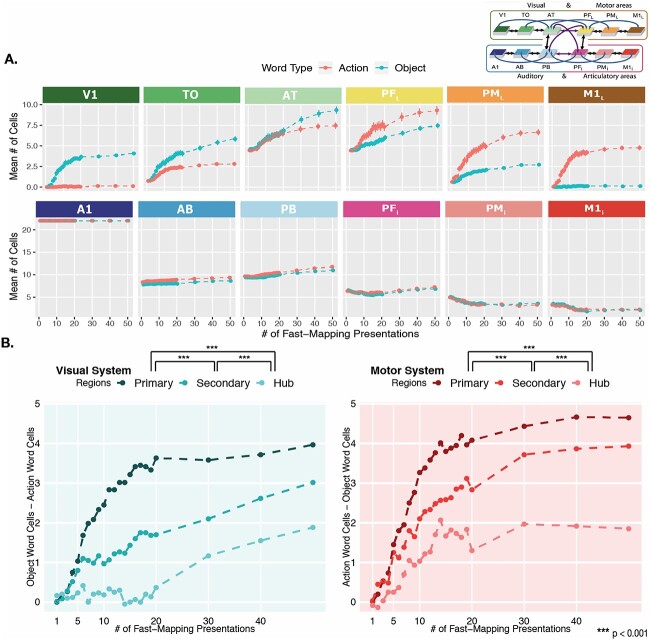
Although teaching animals a few meaningful signs is usually time-consuming, children acquire words easily after only a few exposures, a phenomenon termed "fast-mapping." Meanwhile, most neural network learning algorithms fail to achieve reliable information storage quickly, raising the question of whether a mechanistic explanation of fast-mapping is possible. Here, we applied brain-constrained neural models mimicking fronto-temporal-occipital regions to simulate key features of semantic associative learning. We compared networks (i) with prior encounters with phonological and conceptual knowledge, as claimed by fast-mapping theory, and (ii) without such prior knowledge. Fast-mapping simulations showed word-specific representations to emerge quickly after 1-10 learning events, whereas direct word learning showed word-meaning mappings only after 40-100 events. Furthermore, hub regions appeared to be essential for fast-mapping, and attention facilitated it, but was not strictly necessary. These findings provide a better understanding of the critical mechanisms underlying the human brain's unique ability to acquire new words rapidly.

Keywords: Hebbian learning; biologically neural networks; distributed neural assemblies; fast mapping; language acquisition; semantic grounding.

Fig. 1

Model structure and connectivity. A) The structure and connectivity of the 12 network areas are shown, with the perisylvian articulatory-phonological system in red/pink colors, including primary motor cortex (M1_i), premotor cortex (PM_i), and inferior prefrontal cortex (PF_i), and the acoustic phonological system in blue, including the primary auditory cortex (A1), auditory belt (AB), and parabelt (PB). Extrasylvian regions include the dorsolateral hand-motor system in yellow/brown, consisting of the lateral prefrontal (PF_L), premotor (PM_L), and primary motor (M1_L) cortex, as well as the ventral visual stream in green, including the anterior temporal (AT), temporo-occipital (TO), and primary visual (V1) areas. Numbers refer to Brodmann areas and arrows between areas represent long distance cortico-cortical connections. B) Schematic of the areas and their connectivity structure. C) Micro-connectivity structure of one modeled excitatory “cell,” labeled e. Gray lines arching upward represent within-area excitatory links that are limited to the local neighborhood (light shaded area). Purple lines arching upward capture between-area links. The underlying gray cells represent an inhibitory cell i, which inhibits neighbors proportional to the total input it receives from the neighborhood shaded in darker purple. Figure adapted from Tomasello et al. (2018).

Fig. 2

CAs formed prior to fast-mapping. A) CA examples. Each CA shows the cells belonging to it across the 12 areas, placed on a schematic illustration of the brain with the modeled cortical areas highlighted and color-coded. The color mapping between network areas and brain regions is shown in the schematic in the top right corner. Active cells are depicted as white dots in each gray area. Top-left is an example of the representation of a visual object referent. Top-right is an example of the correlates of a manual action execution. Bottom-left is an example of a phonological word form representation. B) Mean cell counts per area. CA cell counts shown in each area for word forms and referents averaged across 20 networks. Error bars depict standard error (SE). The colored outline of the bars maps them to their respective brain region. Cell counts for the object representations are shown in light gray and cell counts for action representations are shown in darker gray. Word form are later linked with either object or action representations and are split into separate bars on the basis of this future pairing, but the distinction is not meaningful at this point; hence, they all are depicted in gray with tilted stripes. In line with this, pairwise comparisons are only performed and shown for the referents. Depicted P-values have been Bonferroni-corrected. Asterisks illustrate significant differences between the number of neurons in CA circuits of object and action referents.

Fig. 3

Interlinked cell assemblies for word forms and concepts (objects and actions) during fast-mapping. In the far-left and far-right columns, examples of CAs formation after 5 (top), 10 (middle), and 40 presentations (bottom) are shown. Each panel shows the cells activated by stimulating the auditory cortex, area A1 (dark blue), with one auditory word form pattern, which led to the activation of CAs spread across all 12 model areas. These activations are placed on a schematic illustration of the brain with the modeled cortical areas highlighted and color-coded. The color mapping between network areas and brain regions is shown in the schematic in the top-middle. Each gray box shows one simulated area of 625 excitatory cells, with active cells depicted as white dots. The three panels on the left show the CA development for an object word and those on the right that for an action word. Note the activity spreading into extrasylvian visual regions (AT, TO, and V1) for the object word and extrasylvian motor regions (PF_L, PM_L, and M1_L) for the action word, showing successful category-specific fast-mapping. In the middle column, the bar plots show the CA cell counts in each area for action (dark gray) and object (light gray) words, averaged across 20 networks and 3 CAs of each word type per network. This is shown after 5 (top), 10 (middle), and 40 (bottom) learning trials. Error bars depict SE. The colored outline of the bars maps them to their respective brain region.

Fig. 4

Rate of successful word-referent mapping. A) Percentage of rapidly mapped cell assemblies (CAs) across 100 learning trials in one-stage vs two-stage learning. The y-axis depicts, for each learning event, the percentage of CAs per network in which the word form was mapped sufficiently to the referent, allowing for reactivation of at least 10% of the object/action representation in referent extrasylvian areas (V1, TO, and AT for object words and M1_L, PM_L, and PF_L for action words) after auditory stimulation. This is computed across the different learning steps, on the x-axis. Error bars capture SE across networks. B) Proportion of correct vs incorrect referents reactivated across learning trials for two-stage learning. Green points depict the proportion of the correct referent representation that is reactivated after each learning event from just auditory stimulation. Red points depict the proportion of incorrectly activated referent representations, demonstrating that the networks did not make mapping errors. These results are separated by category-specific extrasylvian area, with “primary” corresponding to V1 for object words and M1_L for action words, “secondary” corresponding TO for object words and PM_L for action words, and “hub” corresponding to AT for object words and PF_L for action words. Error bars capture SE across CAs.

Fig. 5

Category-specific topographies across fast-mapping. A) Mean action vs object word CA cells across areas. Emerging category-specific topographical distributions of CAs across learning steps. The y-axis captures the mean number of cells belonging to CAs of that word type, which are calculated specific to each area, at each learning step indicated on the x-axis. Learning steps run from 1 to 50 (with each vertical white line indicating 10). Error bars reflect SE. The schematic in the top-right corner showing the color-coded areas is adapted from Tomasello et al. 2018. B) Category-specificity between region types. The y-axes reflect the difference in mean number of CA cells between the two word types, which serves as a measure of the degree of category-specificity. The left plot in blue depicts the difference between object and action words in extrasylvian visual regions, with the primary region referring to V1, the secondary to TO, and the hub to AT. The right plot in pink depicts the difference between action and object words in extrasylvian motor regions, with the primary region referring to M1_L, the secondary to PM_L, and the hub to PF_L. The significance indicators (^*) at the legends refer to pairwise comparisons between area types collapsed across learning steps, and P-values have been Bonferroni corrected.

Fig. 6

Effect of attention on fast-mapping. A) Mean cell counts per area and attention condition across learning. Emerging distributions of cell counts across learning steps in each attention condition. The y-axis captures the mean number of cells belonging to CAs in each area, collapsed across word-types, at each learning step on the x-axis. The baseline-attention condition reflects the baseline condition in which global inhibition is kept at 0.70 throughout learning (blue line). The high-attention condition reflects a condition in which a global inhibition of 0.50 for the first three learning steps, and then raised to baseline (0.70, red line). Error bars reflect SE. B) Rate of linking per attention condition. The y-axis depicts the percentage out of the CAs per network that have linked such that auditory input reactivates at least 10% of the referent representation in the associated extrasylvian areas (V1, TO, and AT for objects and M1_L, PM_L, and PF_L for action words). This is computed across the different fast-mapping learning steps, on the x-axis. Error bars reflect SE.

References

1. Adams SV, Wennekers T, Cangelosi A, Garagnani M, Pulvermüller F. 2014. Learning visual-motor cell assemblies for the iCub robot using a neuroanatomically grounded neural network. In: 2014 IEEE Symposium on Computational Intelligence, Cognitive Algorithms, Mind, and Brain (CCMB). Presented at the 2014 IEEE Symposium on Computational Intelligence, Cognitive Algorithms, Mind, and Brain (CCMB). p. 1–8.
1. Amir Y, Harel M, Malach R. Cortical hierarchy reflected in the organization of intrinsic connections in macaque monkey visual cortex. J Comp Neurol. 1993:334(1):19–46. - PubMed
1. Arikuni T, Watanabe K, Kubota K. Connections of area 8 with area 6 in the brain of the macaque monkey. J Comp Neurol. 1988:277(1):21–40. - PubMed
1. Artola A, Singer W. Long-term depression of excitatory synaptic transmission and its relationship to long-term potentiation. Trends Neurosci. 1993:16(11):480–487. - PubMed
1. Artola A, Bröcher S, Singer W. Different voltage-dependent thresholds for inducing long-term depression and long-term potentiation in slices of rat visual cortex. Nature. 1990:347(6288):69–72. - PubMed
Publication types