Amorphous entangled active matter

Abstract

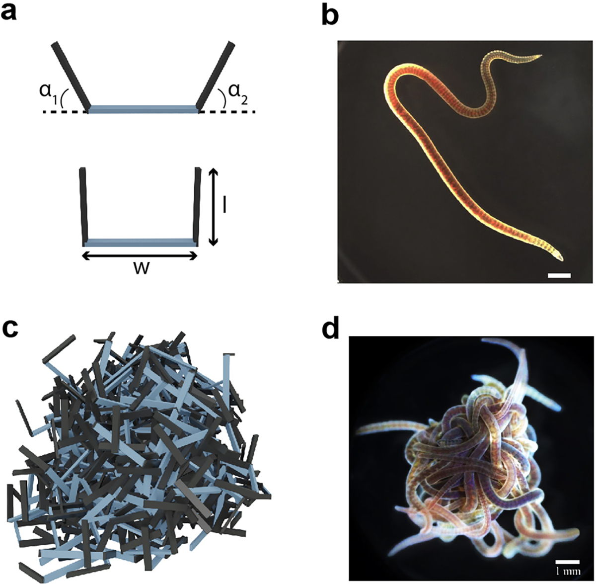
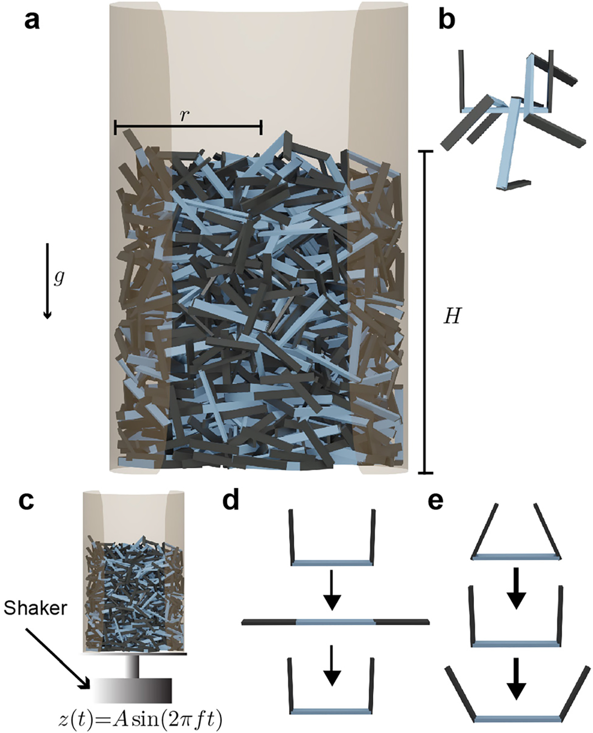
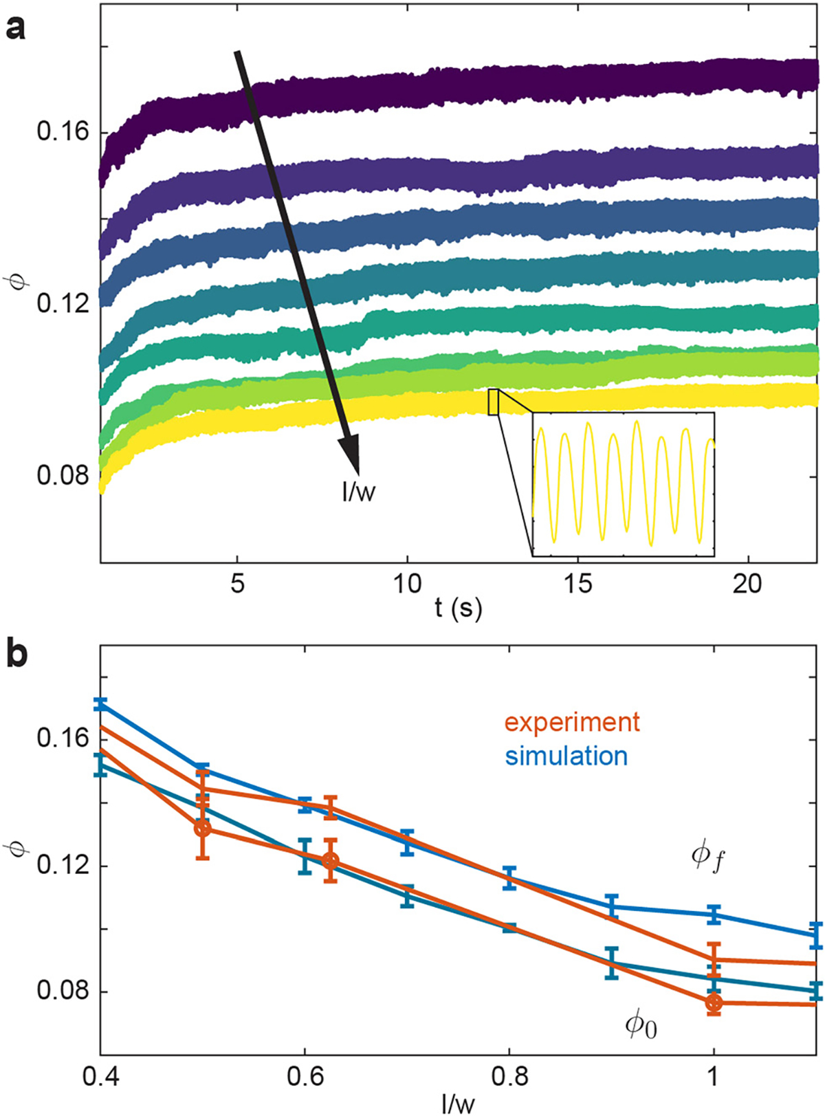
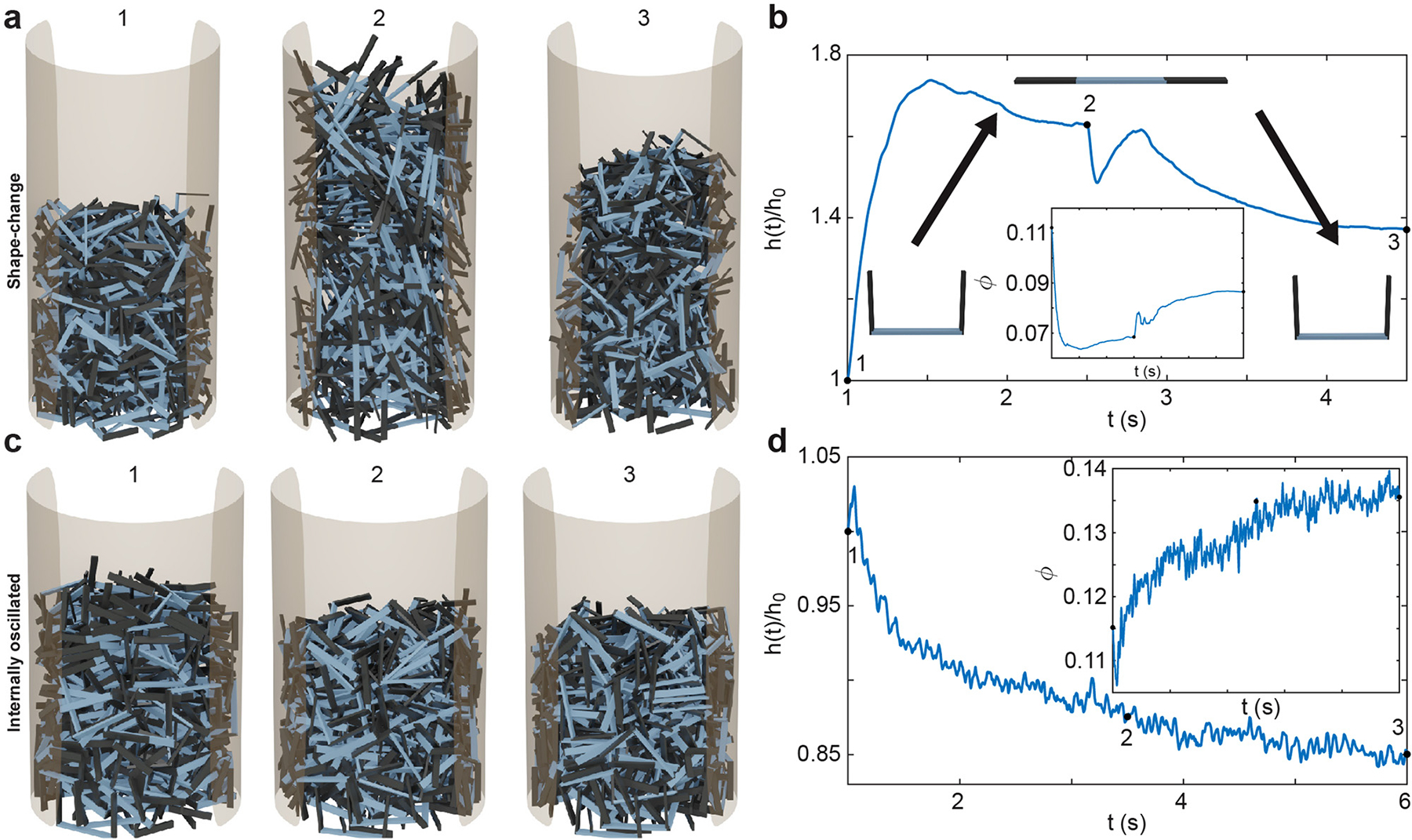
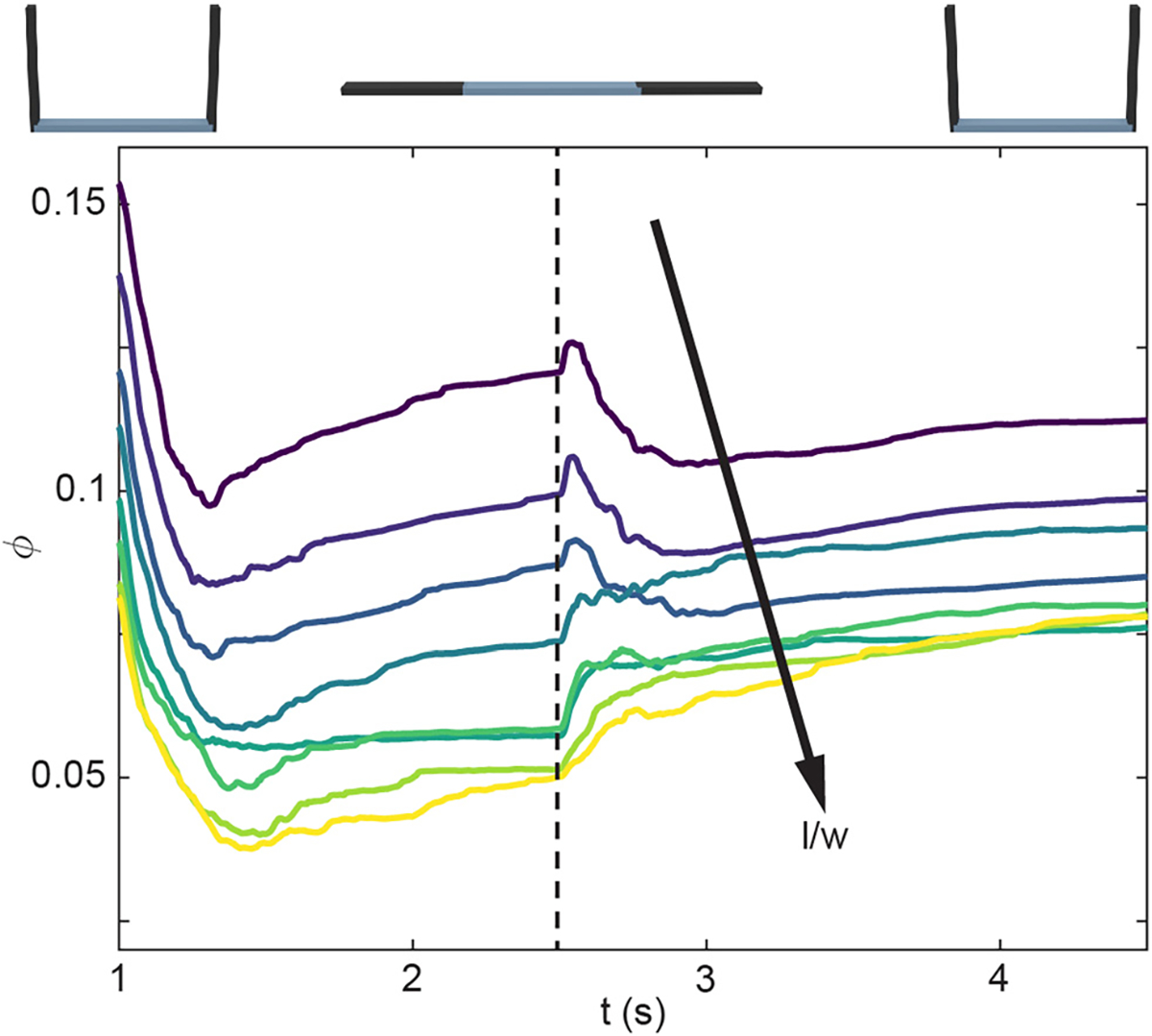
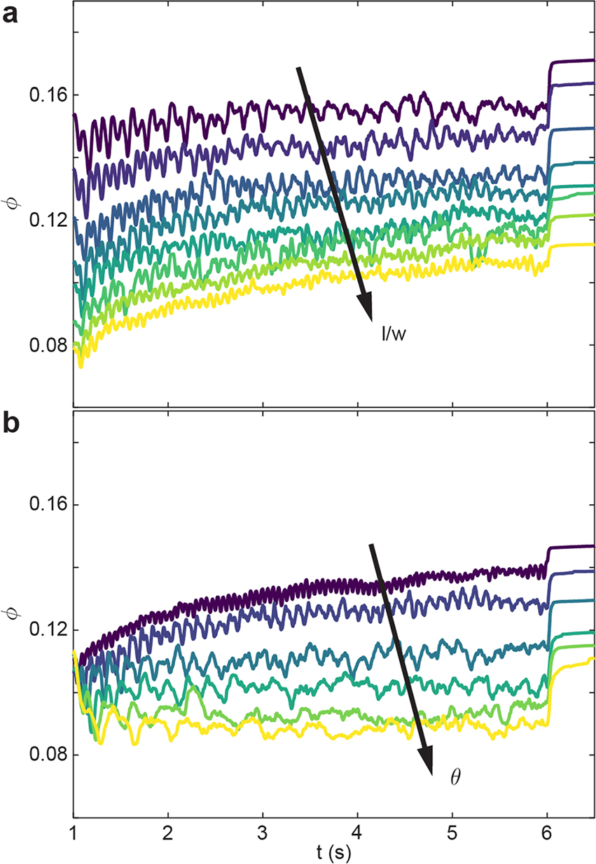
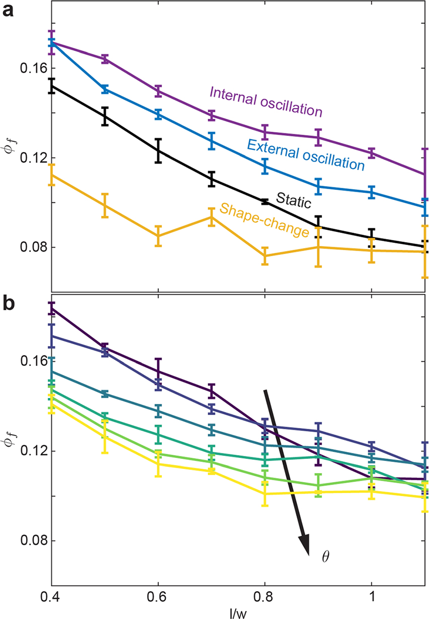
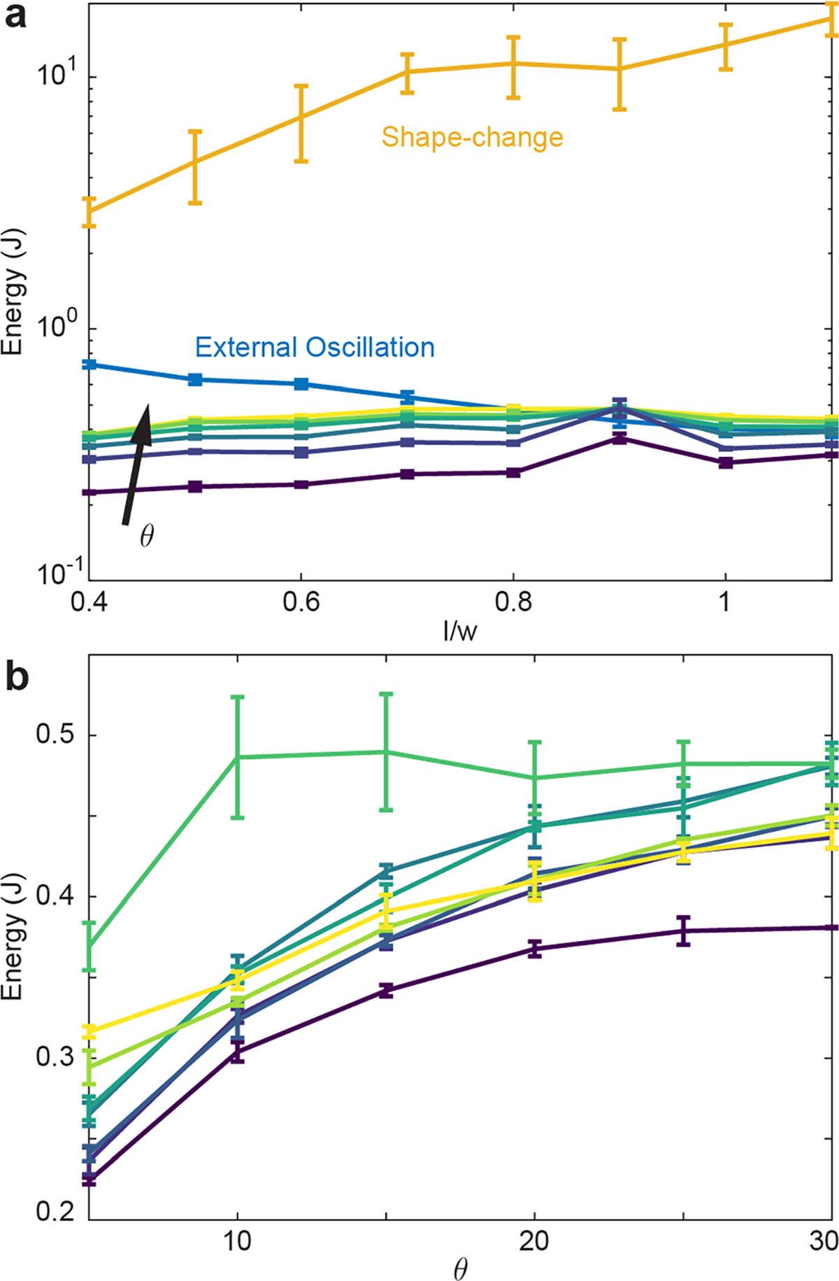
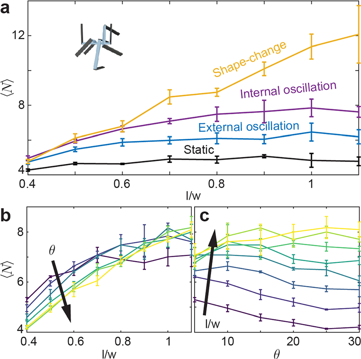
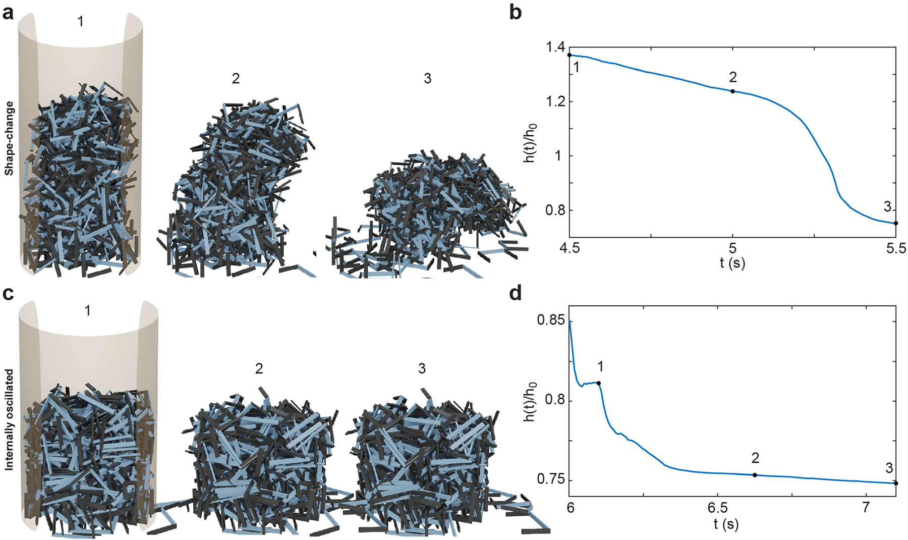
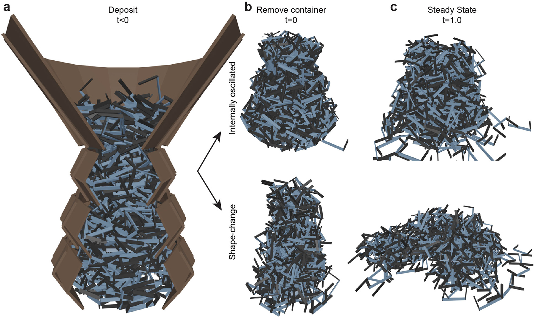
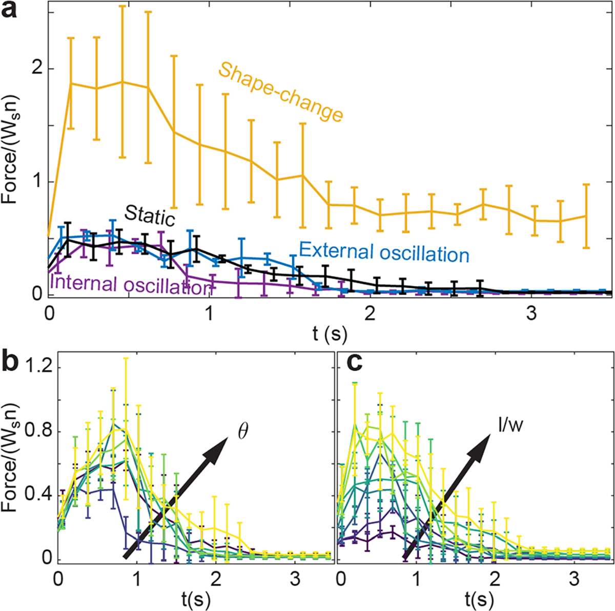
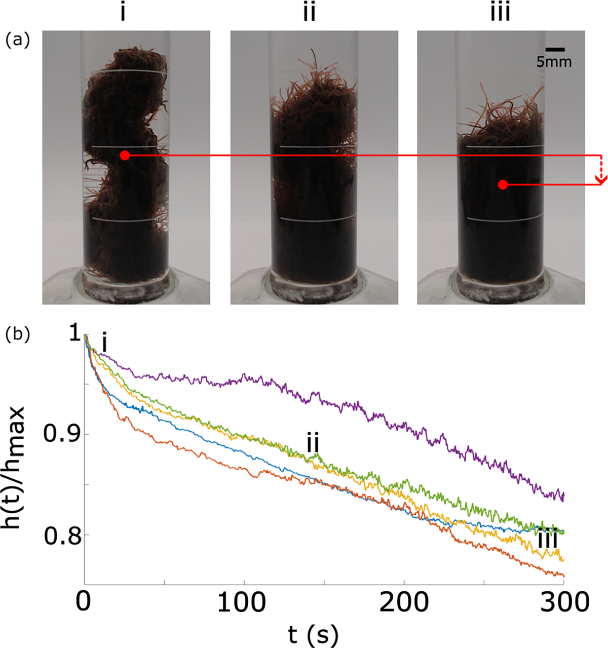
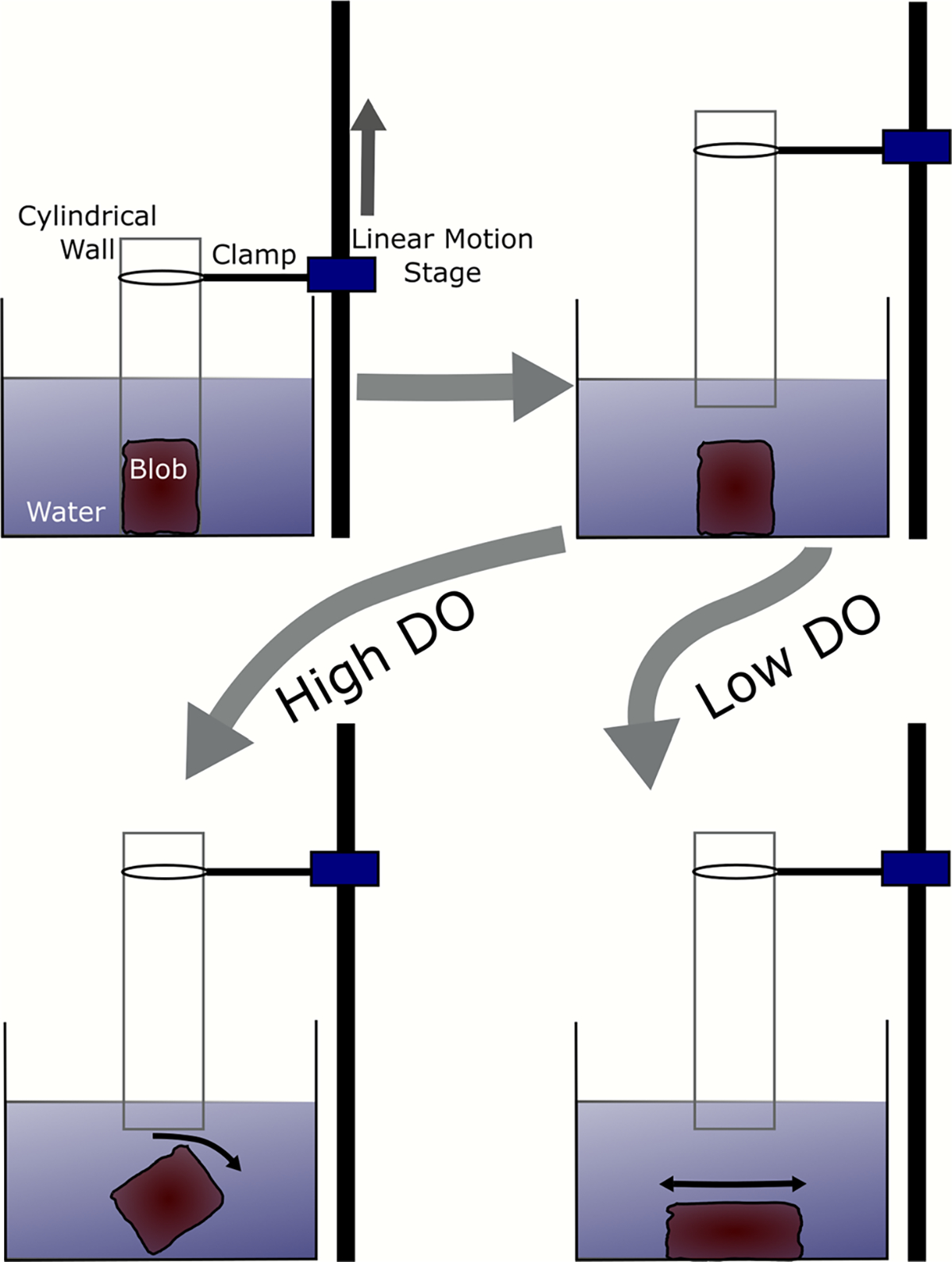
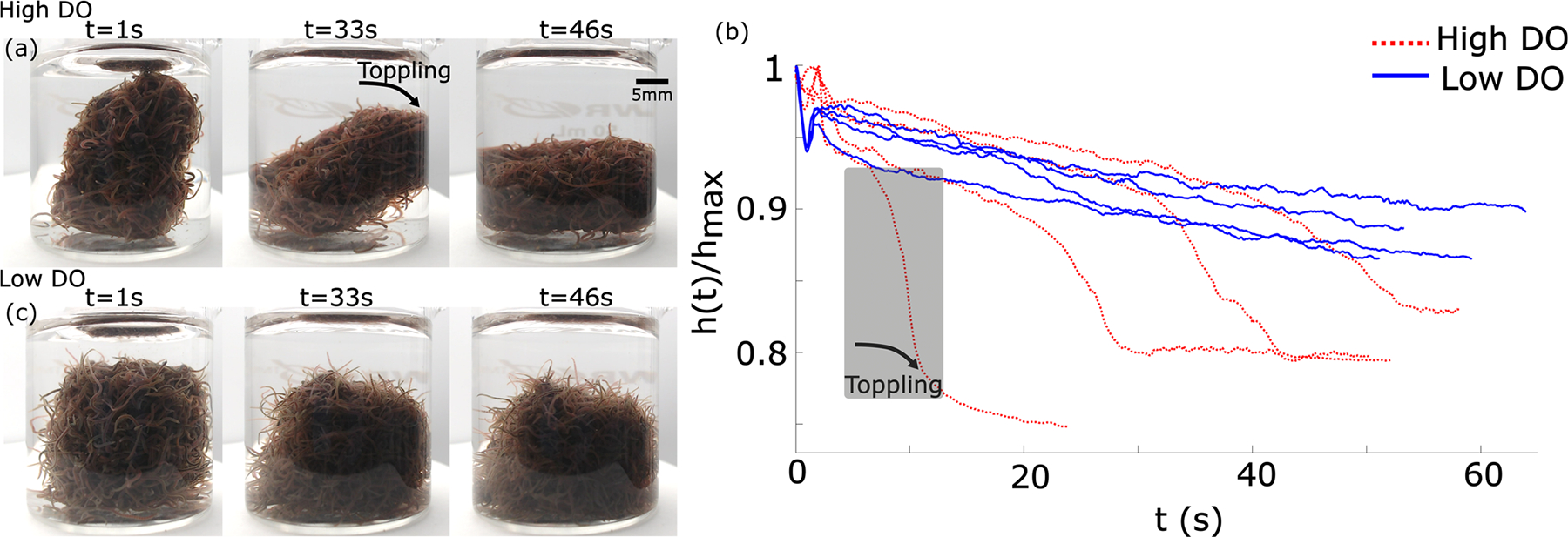
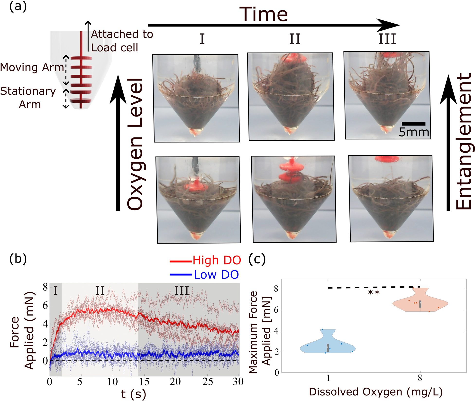
The design of amorphous entangled systems, specifically from soft and active materials, has the potential to open exciting new classes of active, shape-shifting, and task-capable 'smart' materials. However, the global emergent mechanics that arise from the local interactions of individual particles are not well understood. In this study, we examine the emergent properties of amorphous entangled systems in an in silico collection of u-shaped particles ("smarticles") and in living entangled aggregate of worm blobs (L. variegatus). In simulations, we examine how material properties change for a collective composed of smarticles as they undergo different forcing protocols. We compare three methods of controlling entanglement in the collective: external oscillations of the ensemble, sudden shape-changes of all individuals, and sustained internal oscillations of all individuals. We find that large-amplitude changes of the particle's shape using the shape-change procedure produce the largest average number of entanglements, with respect to the aspect ratio (l/w), thus improving the tensile strength of the collective. We demonstrate applications of these simulations by showing how the individual worm activity in a blob can be controlled through the ambient dissolved oxygen in water, leading to complex emergent properties of the living entangled collective, such as solid-like entanglement and tumbling. Our work reveals principles by which future shape-modulating, potentially soft robotic systems may dynamically alter their material properties, advancing our understanding of living entangled materials, while inspiring new classes of synthetic emergent super-materials.

Fig. 1

Smarticles in simulation and a biological analogy. (a) The coordinate system and size designations used for the smarticles. (b) An individual California blackworm (Lumbriculus variegatus). (c) An entangled pile of smarticles in simulation; w = 1.17 cm. (d) A group of 20 individual blackworms forming a physically-entangled blob. Scale bar is 1 mm.

Fig. 2

Various smarticle ensemble activation procedures, internal and external. (a) Render of simulated smarticle system deposited into a closed container of radius $r=2w$, one side is shown open to enhance visualization. (b) Rendering of four smarticles entangled together, here $⟨N⟩=1.5$. (c) In the externally-oscillated procedure, particles were deposited into the container and the container was shaken sinusoidally, parallel to gravity, such that $z\left(t\right)=A\mathrm{s}\mathrm{i}\mathrm{n}\left(2\mathrm{\pi }ft\right)$. (d) In the shape-change procedure, smarticle barbs travelled $\mathrm{\pi }/2$ outwards and returned returned back to the original position, this position change happens a single time in this procedure. (e) In the internal-oscillation procedure, particle barbs oscillated with an amplitude $\theta$ centered around $\left({\mathrm{\alpha }}_1,{\mathrm{\alpha }}_2\right)=(\mathrm{\pi }/2,\mathrm{\pi }/2)$.

Fig. 3

Volume fraction evolution as a function of smarticle aspect ratio under external oscillatory forcing. (a) $\varphi$ vs. time for various smarticles aspect ratios $l/w\in \left[\mathrm{0.4,1.1}\right]l/w\in \left[\mathrm{0.4,1.1}\right]$ The inset is a zoomed in version of the data from $l/w=1.1$ over a 0.25 s domain. (b) $\varphi$ as a function of aspect ratio in experiment (orange) and simulation (blue). The bottom two curves represent the volume fraction before activity was added to the system ${\varphi }_0$ in both simulation and experiment. The top two curves are the final volume fraction after external forcing ${\varphi }_{\mathrm{f}}$. The orange curves were taken from data used in Gravish et al.

Fig. 4

Packing behavior distinctions between two different active procedures. (a) Renders of a shape-change trial at three times. (b) The center-of-mass (CoM), $\frac{h\left(t\right)}{h_0}$, in the z-plane of the shape-change collective, the times of the renders in (1, 2, 3) are highlighted with black points [1s, 2.5s, 4.5s]. (c) Renders of an internally-oscillated trial at three times. (d) The CoM in the z-plane of the internally-oscillated collective, the times of the renders in (1, 2, 3) are highlighted with black points [1s, 3.5s, 6s].

Fig. 5

Evolution of $\varphi$ at different $l/w\in \left[\mathrm{0.4,1.1}\right]$ for the shape-change procedure. Time evolution of $\varphi$ for varying $l/w$ performing the shape-change procedure. The vertical dashed line represents denotes when the “straight” to “u” configuration change begins.

Fig. 6

Time evolution of volume fraction $\varphi$ for various $l/w$ and $\theta$ for the internally-oscillated procedure. (a) $l/w$ is varied $\in \left[\mathrm{0.4,1.1}\right]$ while $\theta ={10}^{\circ }$ is held constant. (b) $\theta$ is varied $\in \left[5^{\circ },{30}^{\circ }\right]$ while $l/w=0.7$ is held constant.

Fig. 7

Final volume fraction ${\varphi }_{\mathrm{f}}$ for the various procedures. (a) ${\varphi }_{\mathrm{f}}$ versus $l/w$ for all procedures. For the internally-oscillated procedure, $\theta ={10}^{\circ }$ was used. (b) ${\varphi }_{\mathrm{f}}$ versus aspect ratio for the internally-oscillated system, each line is has a different $\theta \in \left[5^{\circ },{30}^{\circ }\right]\theta \in \left[5^{\circ },{30}^{\circ }\right]$.

Fig. 8

Comparing energy usage between procedures. (a) Comparisons of energy output for different procedures as a function aspect ratio. The internally-oscillated data are the unlabeled lines where $\theta$ is varied. All data points are averaged from three trials. (b) Energy usage for the internal oscillation procedure as a function of $\theta$ for various aspect ratios. The color gradient here mirrors that used in the earlier figures with purple to yellow being high to low $l/w$.

Fig. 9

Comparing entangling procedures. (a) Comparisons of entanglements for all procedures at various aspect ratios. The internal oscillation line for each point has an amplitude $\theta ={10}^{\circ }$. (b) Entanglement with respect to $l/w$ for the internally-oscillated system $\theta \in \left[5^{\circ },{30}^{\circ }\right]$. (c) Entanglement as a function of $\theta$ for internally-oscillated systems $l/w\in \left[\mathrm{0.4,1.1}\right]l/w\in \left[\mathrm{0.4,1.1}\right]$.

Fig. 10

“Tumbling” and “melting” behavior for active procedures. (a and c) Renders of a shape-change trial and internally-oscillated trial, respectively, at three instances instances. (b and d) The z-plane center-of-mass (CoM) of the collective vs. time, where vs. time, where the three renders from (a and c) are indicated with black points.

Fig. 11

Smarticle aggregate casting and sculpting capabilities. (a) Particles are deposited in in a three-tiered system at $l/w=0.8$ with each tier smaller than the one below. In (b), after the activation state has occurred, (top is internally-oscillated at $\theta ={10}^{\circ }$ and bottom is the shape-change) the outer walls are removed. (c) The piles one second after the container is removed for the internally-oscillated (top) and shape-change (bottom) procedures procedures.(Movie S1, ESI†)

Fig. 12

Measuring tensile and fracture forces as a function of entanglement procedure. Two hooks, colored red, were embedded in an already entangled pile. The force necessary to raise the top hook out of the pile, at constant speed, was measured, while the bottom hook was kept fixed to anchor the pile. Two hooks, colored red, were embedded in an already entangled pile. The force necessary to raise the top hook out of the pile, at constant speed, was measured, while the bottom hook was kept fixed to anchor the pile.

Fig. 13

Tensile force measurements for the various preparation procedures. Force shown here is a unitless quantity scaled by $W_{\mathrm{s}}$, the weight of the smarticles, and $n$, the number of smarticles in the trial. Each line is averaged over 3 trials. (a) Force versus time for the various procedures at $l/w=0.7$, where the peak output force represents the fracture force, (b and c) force versus time for the internally-oscillated system. In (b), $l/w=0.7$ and $\theta$ is varied, and (c) $\theta ={10}^{\circ }$ as varies.

Fig. 14

Evolution of a worm blob from a rigid structure at high concentration of DO to a loosely entangled state in a lower concentration of DO. (a) The red dot depicts the centroid, which move downwards over time as DO is consumed by the worms. Blackworms supplement respiration by disentangling their posterior segments and raising it upwards, emergently relaxing the structure. (b) The normalized height of the blob’s centroid, $\frac{h\left(t\right)}{h_{\mathrm{m}\mathrm{a}\mathrm{x}}}$, plotted as a function of time. Numbers in the time series correspond hmax to the snapshots shown in (a). $n=5$ trials (Movie S2, ESI†).

Fig. 15

The experimental setup for testing the structural stability of the worm blobs under different DO concentrations. Worms were first added into the cylinder then the inner concentric cylindrical wall was lifted up by the linear actuator.

Fig. 16

Tumbling worm blobs. Timelapse of a tumbling worm blob (~8 g) at three instances when present in a (a) high DO and a (b) low DO environment. (c) Timeseries of the normalized height of the blob’s centroid, $\frac{h\left(t\right)}{h_{\mathrm{m}\mathrm{a}\mathrm{x}}}$, over time. $\mathrm{T}=0$ s represents the instance where the inside wall waslifted outside of the water in high DO (blue dotted curves). The gray shaded region indicates the large drop in centroid height when toppling occured for one trial in high DO conditions. $n=4$ trials for each DO levels. (Movie S3, ESI†)

Fig. 17

Experimental setup for blackworms to measure internally-generated forces. (a) Two 3D-printed pieces were placed inside a conical tube: the lower stationary arm was fixed to the bottom to anchor the worms while the upper moving arm was attached to a load cell above. The load cell was attached onto a linear actuator, which allows the upper arm to move in the z-direction. 2 g of worms (N ~ 250) were added into the tube and mixed to allow an even distribution around the arms. The upper arm was gradually raised and the force was measured. The images show snapshots from trials with low DO concentration (bottom row) and high DO concentration (upper row), taken from successive epochs during the trial. (b) Graph of force measured by the load cell as a function of time, for low DO concentration (blue curve) and high DO concentration (red curve). The three epochs I-III in panel (a) correspond to the shaded regions in panel (b). The data points correspond to individual experimental runs and the solid curves are averages across trials. (c) Violin plot of maximum pulling force, in mN, vs. dissolved oxygen level. The solid rectangles indicate the interquartile range while the whiskers indicate the maximum and the minimum value of the distribution. The individual data points are plotted as dots. ** indicate a significance level of 1%. $n=6$ trials for each DO levels.

References

1. Hu D, Phonekeo S, Altshuler E and Brochard-Wyart F, Eur. Phys. J.: Spec. Top, 2016, 225, 629–649.
1. Reid CR, Latty T, Dussutour A and Beekman M, Proc. Natl. Acad. Sci U. S. A, 2012, 109, 17490–17494. - PMC - PubMed
1. Mlot NJ, Tovey CA and Hu DL, Proc. Natl. Acad. Sci U. S. A, 2011, 108, 7669–7673. - PMC - PubMed
1. Ozkan-Aydin Y, Goldman DI and Bhamla MS, Proc. Natl. Acad. Sci U. S. A, 2021, 118, e2010542118. - PMC - PubMed
1. Blackiston D, Lederer E, Kriegman S, Garnier S, Bongard J and Levin M, Sci. Robot, 2021, 6, eabf1571. - PubMed